31 Density-dependence, carrying capacity and vulnerability multipliers
An important feature of Ecosim is that it provides a straightforward approach for exploring alternative views for how the biomass of prey groups are controlled by a predator – or if they are. The two extreme views are “predator” control (also called “top-down”) and “prey control” (or “bottom-up”) – concepts that are quite difficult to fully grasp. But they become really important when you start comparing a model to historical data as a way of establishing credibility of the model’s predictions, because assumptions about them dramatically impact whether the model can “track” or reasonably represent known historical disturbances such as increase in fishing mortality rates. Thus our main attention in both qualitative and quantitative methods for comparing EwE models to data is at least initially on the parameters that determine the pattern of trophic control.
We model this interplay between predator and prey control using “vulnerability multipliers,” which provide a factor for how much an increase in predator abundance may impact the predation mortality that it is causing on a given prey.
- Low vulnerability multipliers (close to 1) mean that an increase in predator biomass will not cause any noticeable increase in the predation mortality the predator may cause on the given prey (see Figure 3.1).
- High vulnerability multipliers, (e.g., 100), indicates that if the predator biomass is for instance doubled, it will cause close to a doubling in the predation mortality it causes for a given prey.

Figure 1. Lesser flamingos in Lake Nakuru, Kenya. Millions of flamingos overwinter in the lake where they feed on brine shrimp (Artemia) in the shallow parts of the lake. Do flamingos control the prey population? Or is it the productivity of the Artemia population that determines how much the flamingos get to eat? Would twice as many flamingos eat twice as many Artemia?
On carrying capacity
When a predator is at its carrying capacity, its production depends on how productive its prey populations are. If it’s a good year in the environment with high prey production, there will be more food for the predator – and its carrying capacity may increase. Vice versa if productivity is low. How much a predator population gets to eat depends on how productive their prey populations are. So, when a predator is close to its carrying capacity the system is “bottom-up” controlled. In this case, the Ecosim vulnerability multipliers are low, close to 1.
If the predator is far from its carrying capacity, the predator has very little control over its prey populations (there are too few of them!), but it’s called “top-down” control because how much the predators eat depends on how many predators there are (rather confusing, eh?) Twice as many predators may eat twice as much food (and hence cause twice as high predation mortality) but have no notable impact on the prey population (still, it’s called “top-down” control). Here, we need to use high vulnerability multipliers in Ecosim.
You can think of it like this. The vulnerability multiplier sets how many times the predation mortality a predator is causing on its prey may increase if the predator population were to increase to its carrying capacity. If that multiplier is 100, then the predator is far from its carrying capacity – the population can perhaps grow >100 times before reaching carrying capacity. “>100” because the competition between the predators will be intense when they are at carrying capacity, so the average individual will get less food than if their population was much lower.
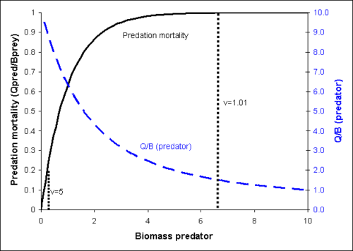
Figure 2. Relationship between biomass of a predator and the predation mortality it causes on a given prey, as well as the corresponding Q/B for the given predator and prey (assuming that the predator does not reduce prey biomass substantially). Vulnerability multipliers, v, are estimated as max. predation mortality/baseline predation mortality, (e.g., 5 at the left-most stippled line). Baseline mortality is the mortality caused by the predator in the underlying Ecopath model.
If we illustrate the relationship between predator biomass and Q/B (this is not an assumption in the actual Ecosim calculations) and assume that the predator in question does not cause any substantial (actually no) change in the prey biomass, we can calculate the relative Q/B for the predator (see Figure 2). For higher predator biomass, a change will result in relatively stable predation mortality. Hence, if biomass is impacted so as to cause a reduction, the individual predators will get more, their Q/B increase and this will largely compensate for the reduction in their abundance, bringing the biomass back up again.
At lower biomass, Q/B will also increase, but to a lower degree. This is illustrated in Figure 3 showing how halving or doubling the predator biomass will impact the relative Q/B. At high biomasses, halving biomass results in close to a doubling in Q/B, which will tend to keep biomass high. There is, however, less and less relative surplus production as we move to the left on the curve. If biomasses are doubled instead, the Q/B will decrease when biomasses are high, resulting in a decrease in biomass back toward the original level, i.e., the biomasses will be stable when close to carrying capacity (where v’s are low), and unstable when far below carrying capacity (where v’s are high).
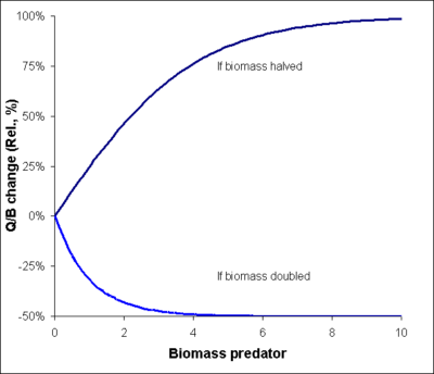
Figure 3. Relative increase (%) in Q/B as a function of predator biomass resulting from the predator biomass being halved or doubled. At high predator biomasses (i.e. near the carrying capacity for the given predator-prey interaction) a halving of predator biomass will result in nearly a doubling in the Q/B for the predator. The resulting surplus production will tend to bring the predator biomass back to the original level, and the overall effect is that the predator biomass will change only little. Conversely, a doubling of predators will cause the Q/B to be halved at high predator biomasses (resulting in very little effective change in biomass), while a doubling at low biomasses will result in only a very small reduction in Q/B.
If vulnerabilities are high, the amount of prey consumed by the predator is the product of predator times prey biomass, i.e., the predator biomass directly impacts how much of the prey is consumed. Such situation may occur in a situation where the prey has no refuge, and is thus always taken upon being encountered by a predator. Such top-down control, also known as Lotka-Volterra dynamics, easily leads to rapid oscillations of prey and predator populations and with it, making it impossible to maintain prey populations in a model.
In Ecosim, however, top-down control implies that a predator is far from its carrying capacity. Hence, if there’s only a small predator population around and conditions (available food, mortality reduction) allow it, the predator population may grow towards its carrying capacity. How much it may grow, given favourable conditions, depends on the vulnerability multiplier.
If you are modelling an area where a predator population is close to its carrying capacity – maybe something like Kingman Reef where apex predators make up 85% of the total fish biomass – then those predators depend on how productive the prey population is. More predators does not mean more prey consumption, the system is bottom-up controlled, and vulnerability multipliers should be low for such predators. This is a stable ecosystem configuration. If a burst of fishing should occur at Kingman Reef, those fish that are left will see improved prey conditions, their Q/B will increase, and the population will grow back towards its carrying capacity.
Bottom-up control can also occur where a prey is protected most of the time, (e.g., by hiding in crevices) and becomes available to predators only when it leaves the feature that protects it. Here being caught is a function of the prey’s behaviour. Bottom-up control implies stable system conditions, so it’s associated with only small biomass changes in the prey and predator(s) concerned for instance as a function of fishing pressure.
The converse (top-down control) is the situation that occurs when a predator population is far from its carrying capacity – for instance because the population has been fished to the brink. In this situation, there are only few predators around and their prey populations may have increased due to predator release or cascading.
To model this interplay between top-down and bottom-up control in predator-prey interactions, the group biomasses in the underlying Ecopath model were in the foraging arena theory[1] [2] [3] [4] in Ecosim conceived as consisting of two components, one vulnerable and one invulnerable to predation. We’ll discuss this in more detail in the next chapter.
Model behaviour depends strongly on the vulnerability multipliers. How do you set those then? The most common way is to fit the model to time series data, which may imply fitting to vulnerabilities along with environmental productivity (see chapter). It worth remembering though that the vulnerability multipliers are not “nuisance parameters” (i.e. parameters which have no specific interpretation), but express how far a predator population is from its carrying capacity
Vulnerability multiplier = how many times might this predator increase the predation mortality it’s causing on its prey, if it were to grow to its carrying capacity?
Carrying capacity is not constant; in Ecosim the vulnerability multipliers are relevant for and used only in the Ecopath baseline. Carrying capacity may then change for each and every time step in Ecosim if need be. Ecosim considers that and populations may change accordingly.
If you reflect on figures such as Figures 2 and 3, note that the x-axis is biomass. That implies we are talking about density-dependence, how much impact a predator has on its prey populations and how much a predator gets to eat is density-dependent.
Quiz
Media Attributions
- Large_number_of_flamingos_at_Lake_Nakuru adapted by Licensed under the Creative Commons Attribution-Share Alike 3.0 Unported, 2.5 Generic, 2.0 Generic and 1.0 Generic license.
- Walters, C. J. and F. Juanes (1993). Recruitment limitations as a consequence of natural selection for use of restricted feeding habitats and predation risk taking by juvenile fishes. Can. J. Fish.Aquat. Sci. 50, 2058-2070 ↵
- Walters, C. J. and J. Korman (1999). Linking recruitment to trophic factors: revisiting the Beverton-Holt recruitment model from a life history and multispecies perspective. Rev. Fish Biol. Fish. 9, 187-202. ↵
- Walters CJ, SJD Martell. 2004. Fisheries Ecology and Management. Princeton University Press. ↵
- Ahrens, R. N. M., Walters, C. J., and Christensen, V. 2012. Foraging arena theory. Fish and Fisheries 13: 41–59. ↵
