2 Modelling predator-prey interactions

On the path to ecosystem-based management: species interactions

Let there be no doubt, single species assessment is a necessary factor for management of fisheries, notably for tactical management. How do we manage this species in this bay this year? What we need to ask, however, is if it is sufficient?

Views on this question go back a long time as expressed by the two pioneers that more than any established fisheries science as a quantitative discipline, Ray Beverton and Sidney Holt. In their 1957 Magnus Opus, “On the Dynamics of Exploited Fish Populations”^[1] they wrote (p.24):

“Elton (1949) has suggested that the goal of ecological survey is ‘…to discover the main dynamic relations between populations living in an area’. This is a generalization of what is now perhaps the central problem of fisheries research: the investigation not merely of the reactions of particular populations to fishing, but also of interactions between them and the extent to which it is possible and practicable to derive laws describing the behavior of the community from those concerning the properties of component populations”

Ray Beverton and Sidney Holt in their book set the vast part of the agenda that fisheries scientists have worked on ever since. So is the case for species interactions as the quote above illustrates.  If the assessments are short-term, as single species assessments tend to be, we can get by assuming “business as usual”, but when we move away from the initial state, i.e. when we address questions at the ecosystem-level we have no choice.

“Fish eat fish“, Erik Ursin – who along with K.P. Andersen created one of the first end-to-end ecosystem models^[2] – often said. And yes, fish eat fish, and that has implications for management of living resources in aquatic environments. If we are to successfully manage ecosystems, then species interactions is part of the foundation.

The foundation for this was laid a century ago, when Lotka^[3] and Volterra^[4][5] both and independently formulated a theory for predator-prey interactions. Models based on these sources are called Lotka-Volterra models and they are in essence the foundation for all predator-prey models, including the dynamic models in EwE.

The basis is that with no resource limitations and no predators, prey populations (N) will change over time with an exponential growth rate (r),

[latex]dN/dt=rN \tag{1}[/latex]

and predator populations (P) will decrease with a mortality rate (m, due to e.g., starvation or old age),

[latex]dP/dt=-mP \tag{2}[/latex]

In a simple predator-prey system with no resource limitations for prey, the equations can be coupled. For the prey population, we describe the change over time with the differential equation,

[latex]dN/dt=rN-aNP\tag{3}[/latex]

where the factor a is called the search rate. For the predator,

[latex]dP/dt=gaNP-mP\tag{4}[/latex]

where g is the growth efficiency with which the predator converts consumption to production.

If you examine these equations carefully, you’ll notice that the predator’s consumption (Q) is calculated as

[latex]Q=aNP\tag{5}[/latex]

which means that more predators (P) lead to more predation, and more prey (N) means more predation – the consumption is the product of the two and the search rate constant.  Systems modelled with such assumptions are unstable, initially the predator population may grow if there are plenty of prey around, but as it grows, the prey population gets more impacted and at some point the prey will collapse. The slower-growing predators will survive for a while, but in a simple two species systems, they will eventually collapse as well. That in turn releases predation mortality from the minuscule prey populations, which will have great conditions and start growing exponentially – after which history repeats itself, the predator will increase, the prey collapse, the predator collapse. The system becomes cyclic and unstable.

The cyclic and unstable nature of Lotka-Volterra systems is not what we see in most ecosystems, and for that reason there have been numerous modifications proposed, notably after C.S. Holling^[6]  added predator handling time (h) through his disk equation where the consumption by a predator is estimated as,

[latex]Q=aNP/(1+hN)\tag{6}[/latex]

recognizing that the time a predator spends handling a prey it will not be searching for new prey. That limits the predator consumption rate at high prey densities – and leads immediately to unstable dynamics (exploding cycles) in the predictions unless some other factor(s) are included in the model to limit variation in prey and/or predator abundances and predation rates.

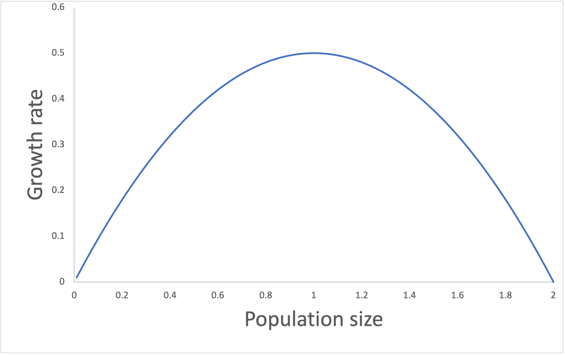
Figure 1. Population growth as a function of population size for the logistic (Verhulst) model. Carrying capacity for the population is set at 2.

Lotka-Volterra models can be defined without (as above) or with resource limitation, i.e. carrying capacity (K). The “standard” way of implanting resource limitation is to express prey population change using the logistic equation for population growth (Verhulst),

[latex]dN/dt=rN(1-N/K)\tag{7}[/latex]

Foraging arena

The foraging arena theory was developed by Carl Walters, and serves as the foundation for the dynamic modules of EwE, i.e. of Ecosim and Ecospace. The basic assumption in foraging arena theory is that spatial and temporal restrictions in predator and prey activity cause partitioning of prey populations into vulnerable and invulnerable population components, such that predation rates are dependent on (and limited by) exchange rates between these prey components^[7].

Foraging arena models (such as Ecosim^[8]) are based on Lotka-Volterra modelling but the interaction terms only include the vulnerable part (V) of the total prey population (N). So, where we for Lotka-Volterra models have the predator consumption (Q) estimated from,

[latex]Q=aNP\tag{8}[/latex]

the similar equation for foraging arena models is,

[latex]Q=aVP\tag{9}[/latex]

Further, the prey exchange between vulnerable and in vulnerable states can be described with the rate equation,

[latex]dV/dt=v(N-V)-v'-aVP\tag{10}[/latex]

from which V is predicted to the moving equilibrium (for N and V), setting dV/dt to 0,

[latex]V=vN/(v+v'+aP)\tag{11}[/latex]

Changes in the predator and prey populations over time can then be predicted from the Lotka-Volterra model equations, substituting the total prey populations (N) with the vulnerable population (V).

Associated tutorial

There is a tutorial to accompany this section in the next chapter of the web version of this book. You can either develop a Lotta-Volterra model based on the equations above or use the R-code that is included in the tutorial (or do both).

Quiz