14 Foraging arena theory
Robert NM Ahrens; Villy Christensen; and Carl J. Walters
Foraging arena theory is the driving machinery in EwE, and it represents a development that has had profound implications for making ecosystem models behave, be able to replicate the ecosystem history and make plausible predictions. Without the foraging arena theory there would be no EwE.
The foraging arena theory emerged through a series of studies during the 1990s[1] [2] [3]. The general predictions of foraging arena theory have been fairly widely used by fisheries scientists, mainly through the application of EwE-Ecosim, to explain and model responses of harvested ecosystems[4]. The potential for the underlying ecological theory upon which foraging arena theory is based to help to understand a broad range of aquatic ecosystem behaviours has apparently not been widely recognized.
Here we describe the basic models of foraging arena theory. We review the various mechanisms that can lead to these models, list the main predictions they imply, and give an overview of the practical difficulties that have been encountered in estimating critical vulnerability exchange rate parameters that appear to limit trophic interaction rates. The present chapter is an adapted extract from Ahrens et al.[5] to which we refer for a fuller presentation and notably examples with references.
Basic models of foraging arena theory
The basic assertion of foraging arena theory is that spatial and temporal restrictions in predator and prey activity cause partitioning of each prey population into vulnerable and invulnerable population components, such that predation rates are dependent on (and limited by) exchange rates between these prey components. Trophic interactions take place in the restricted "foraging arenas" where vulnerable prey can be found (Figure 1 and 2).
That is, if the total prey population is Bi, and Vi of these are vulnerable to predation at any moment (i.e. are in the foraging arena for interaction with some predator whose abundance is Bj), total prey consumption rate Qj should be predictable as the mass action product
[latex]Q_j=a_{ij} \ V \ B_j \tag{1}[/latex]
where the predator rate of effective search aij has units of area or volume per time searched by the predator divided by the area or volume (A) of the foraging arena. Note here that Qj is predictable as Qj=aij Bi Bj only when Vi=Bi, i.e. when all Bi prey and Bj predators are randomly distributed or well-mixed.

Figure 1. Aquatic organisms have evolved a diversity of behaviours that limit their exposure to predation risk. The use of spatial refuges from predation is likely to restrict foraging to limited volumes (V) nearby and limit predator-prey interaction.
This argument remains the same if the predator exhibits type II behaviour, i.e. if aij is reduced when search time is lost due to prey handling[6] [7]. We might represent such effects for example with the multispecies disc equation[8].
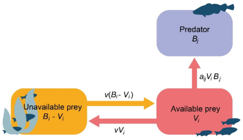
Figure 2. Simulation of flow between available (Vi) and unavailable (Bi– Vi) prey biomass in Ecosim. aij is the predator search rate for prey i, v is the exchange rate between the vulnerable and invulnerable state. Fast equilibrium between the two prey states implies Vi= vBi/ (2v + aBj).[9]
Two specific models have been proposed for predicting changes in vulnerable prey densities V in foraging arenas[10]. The first or "continuous exchange" model[11] proposes that prey exchange between the vulnerable and invulnerable states at instantaneous rates v and v′, so that Vi gains individuals at rate v(Bi-Vi) and loses them at rates v′Vi and aViBj. This results in the rate equation
[latex]dV_i/dt=v(B_i-V_i)-v' \ V_i - a_{ij}V_i \ B_j\tag{2}[/latex]
If the vulnerability exchange and predation rates are high compared to overall rates of change of Bi and Bj, Vi is predicted to remain close to the moving equilibrium (with Bi and Bj) given by solving Eq. 2 with dVi/dt=0:
[latex]V_i=vB_i/(v+v'+a_{ij}B_j)\tag{3}[/latex]
The second or "bout feeding" model proposes that prey (or predators) regularly (e.g., daily at dawn and dusk) enter the foraging arena for short temporal feeding bouts, depleting Vi exponentially during each bout such that the mean prey density seen by the predator during each bout of duration T is given by
[latex]V_i=vB_i(1-e^{-aB_jT}/a_{ij} B_j )\tag{4}[/latex]
and initial vulnerable prey abundance vBi is some fraction of the total prey population Bi. Note that both of these models imply two alternative ways to precisely define the phrase "limited food supply", found in ecological arguments[12], but generally lacks a formal definition. The supply of food may be defined as a temporal rate vN of food delivery to foraging arenas, or alternatively as the limited food density V that results from the balance of supply rate and removal processes.
An immediate and crucial prediction of models represented by Eq. 3 and Eq. 4 is that there can be strong negative effect of predator abundance Bj on vulnerable prey density Vi and feeding rate per predator Q/Bj, whether or not predators have any substantial impact on total prey abundance Bi[13]. Substituting Eq. 2 into Eq. 1 results in the "functional response" prediction
[latex]Q/B_j = a \ v \ B_i/(v+v'+a B_j)\tag{5}[/latex]
That is, the basic foraging arena models predict strong "ratio dependence" in the predation rate Qj, with attendant consequences for predator-prey stability. Further, these models do not depend on specific assumptions about predator behaviour, such as interference or contest competition. Unlike models based on substituting Bj/Bi (prey per predator) ratios into functional response models they can be derived from fine-scale arguments about behaviour and spatial organization of interactions, and so are not subject to Abrams[14] very valid criticisms about the simplistic ratio formulations. Foraging arena models assert that competition between predators is intensified from the spatial restriction of interactions into arenas, however there is no one factor that restricts foraging activity, and restriction may arise result from factors such as prey and/or predator behaviours, or specific habitat requirements. Another basic prediction is that interaction rates Qj can vary between "bottom-up" controlled and "top-down" controlled depending on v and aij. This is easiest to see with Eq. 2: If v is small and aij is large, Qj approaches the "donor controlled" limiting rate vBi as Bj increases; but as v increases, Qj approaches the mass action rate aijBiBj.
The predictions from the foraging arena equations extend across a wide range of scales. Before describing these predictions in more detail, we find it important to demonstrate that the fundamental assumption of partitioning of prey into Vi and Bi-Vi components, with attendant exchange processes that can limit trophic interactions, is very widespread or potentially universal at least in aquatic ecosystems. Partitioning resulting from exchange processes implies a basic reversal of the idea that small proportions of prey may be in safe refuges so as to cause predation rates to have type III functional response form. Under the foraging arena assumption, it is far more common for the bulk of prey to be in refuges at any moment, particularly when exchange rates are low. Intense completion for resources within the foraging arena potentially results in increased foraging times by prey[15] as prey density increases, resulting in the type III form of the functional response due to changes in prey behaviour rather than predator behaviour.
Mechanisms that cause prey population partitioning and vulnerability exchange processes
A critical point about vulnerability exchange structures is that restriction in activity by any one species is likely to induce the exchange structure represented by Eq. 1 for at least two trophic linkages, between the species and its prey and between the species and its predator(s). Consider for example the simple food chain zooplankton [latex]\rightarrow[/latex] small fish [latex]\rightarrow[/latex] piscivore. If the small fish "chooses" to restrict its activities so as to forage only near hiding places, most of the small fish become invulnerable at any moment to piscivores. Likewise, then most of its zooplankton prey population becomes invulnerable to it at any moment. This "cascade" of foraging arena structures results in spatially limited interactions between predator and prey occurring on time scales of minutes/hours and at the spatial scale of meters (Figure 3), intensifying competition between predators when exchange processes limit the rate at which prey are replenished.
 Figure 3. Foraging arena predictions across a range of space/time scales. The restriction of predator-prey interaction to "foraging arenas" results in a decreasing hyperbolic relationship between available prey density (Vi) and predator density (Pj) at fine space/time scales. Intra-specific competition within these arenas leads to the commonly observed Beverton-Holt recruitment relationship. For inter-specific interactions, the exchange of prey into and out of these arenas limits predation mortality resulting in community stability. Bi is total prey biomass.
In the following section, we present a simple classification of behaviours that can lead to vulnerability exchange dynamics is presented. This classification is not complete or exhaustive, but it does cover a wide variety of trophic interactions in aquatic systems and demonstrates the broad applicability of foraging arena theory, (for relevant examples in the literature, see the source publication).
1. Arena structure caused by restricted spatial distribution of predators relative to prey
This category includes the original situation mentioned above, where the predator distribution covers only a small proportion of the area or volume occupied by prey organisms. But such restricted overlap can be caused by a variety of factors of which two appear to be particularly common. In all such cases, the vulnerability exchange rates v and v′ are likely to have values determined mainly by physical transport (advection, diffusion) and random movement processes of the prey, and can be extremely low proportions of the overall prey population in physically large systems.
1.a. Restricted predator distribution in response to predation risk caused by its predators
The behaviour of post-larval juvenile fish is likely dominated by a need to reduce predation risk, and this is likely also the case for juveniles of mobile invertebrates. So far as we know from many examples, post-larvae move into highly restricted habitats (e.g., structure, schools) and spend relatively little time foraging. For most fish, increase in body size is associated with ontogenetic habitat shifts to use much larger foraging arenas and multiple habitat types.
Many mobile aquatic invertebrates exhibit strong vertical migration behaviours, apparently in response to predation risk but perhaps also as a way to manage metabolic costs or gain a horizontal transport advantage. Such behaviours result in temporally limited periods of overlap with prey, leading to diurnal foraging bouts and possibly localized prey depletion as represented by Eq. 4.
1.b. Restricted predator distribution caused by limited predator mobility or habitat requirements
Many "predators" have limited or no mobility, for example sessile invertebrates that filter-feed the water column above their resting site. Such restriction in vertical access to prey obviously creates a foraging arena exchange structure with algal and detritus "prey" distributed over the whole water column.
In some cases, apparently mobile predators still concentrate their activities in particular habitats even when not faced with obvious predation risk, perhaps as a way to manage energetic costs and/or places for ambushing prey. Many reef and demersal fish tend to hold and forage near bottom structure, even while taking mainly planktonic prey; one reason for this is that the ocean bottom acts as a trap to concentrate vertically migrating prey species. Such behaviour may be optimal under certain conditions and establishes an arena type structure.
2. Restricted prey distribution and/or activity
This category represents situations where predators may be widely distributed, but their prey show possibly severe restriction in spatial distribution and activity. Predators that exhibit type 1.a. behaviour above with respect to their prey are in turn expected to exhibit type 2 behaviour with respect to interactions with the species that prey on them.
2.a. Time allocation to safe/resting sites
This is the interesting case from an evolutionary perspective, where the same behaviours used to acquire resources (movement into foraging arenas to feed) cause some creatures to be the resources of other species (predation risk concentrated in the same arenas). Obviously such situations create trade-off relationships for which we can expect strong natural selection for optimized time allocation. It is difficult to generalize about the amount of time spent individuals under predation threat spend in refuge habitats. There is an indication that for juvenile fish, the optimum appears to typically be a small-time allocations to foraging particularly when foraging is restricted to crepuscular periods.
2.b. Vulnerability exchange associated with dispersal behaviours
The acquisition of resources is not the only behaviour that can expose organisms periodically to predation risk. Dispersal behaviours are also dangerous, and can occur for a wide variety of reasons (ontogenetic changes in habitat requirements or opportunities, response to locally high densities of competitors, movement to reproductive sites, etc.) Perhaps the most obvious example in aquatic systems is drift of benthic stream insects that spend most of their time in interstitial microhabitats where they are safe from most fish predation, but occasionally leave such sites to drift downstream. In this case, the V of Eq. 1 is literally the concentration of drifting (and emerging) insects, and the drift entry rate v can be limiting to potential abundance of stream predators like trout.
2.c. Vulnerability exchange caused by agonistic behaviours
Many aquatic organisms defend restricted resting or mating sites, and exhibit strong aggressive behaviours toward nearby conspecifics. In such cases, there can be strong density-dependent increase in agonistic activity with increasing density of conspecifics, leading to increased predation risk and density-dependent mortality at high densities.
2.d. High proportion of individual mass not accessible or digestible
Some predators take only parts of their prey without normally killing the prey. For example, browsing herbivores often select only particular plant parts that are physically accessible (not too high off the ground, not underground) or high in quality (seeds, leaves and active growth tips that are high in protein), leaving most of the prey growth/production system intact. In such cases, the v process represents prey body growth. Such dynamic structures are much more common in terrestrial than aquatic environments, but they do occur with grazers on macrophytes and macroalgae, and even with animal-animal interactions like fishes that nip at the siphons of buried molluscs or "graze" on parts of corals.
3. Spatial displacement of predators and prey by physical transport processes
It is common in aquatic ecosystems for production dynamics to be ordered in a physical flow pattern, where nutrient delivery at the head of the flow gives rise to primary production peaks downstream some distance (as primary producers are advected away from the nutrient source as they grow), and to secondary production peaks still further downstream as animals grow in response to the primary production as they are advected.
In such flow structures, smaller organisms may be able to partially control their downstream positions through counter-current movements (vertical migration, emergence and flying upstream). If these behaviours are not completely successful at bringing organisms to centers of prey abundance, such counter-current movements can result in organisms being concentrated in areas along the flow such that their food species appear to exhibit largely donor-controlled dynamics, i.e., to have concentration dynamics V with the same dominant terms (exchange in and out, predation loss) as in Eq. 1.
A similar concentration dynamic is observed when physical flow processes concentrate organism at frontal zones. These areas of higher food concentrations appear to be important foraging areas for higher trophic level organism such as sea birds or whales. In these structures, the concentration of production from a much wider areas establishes a foraging arena as organism exchange into frontal areas either through physical transport or directed movement.
Foraging arena predictions for a range of scales
A fundamental assumption of foraging arena theory is that predator-prey interactions occur at the scale of hours and meters through various behavioural and physical mechanisms potentially restricting prey exposure to predation and intensify competition between predators. This foraging arena formulation provides a structure that can be used to predicting observed states across a range of scale from the individual up to the ecosystem level.
At the scale of the individual, foraging arena theory can be invoked to explain the failure of fishes at least to consume nearly as much food as we would predict to be possible based on large-scale sampling of prey abundances. Back calculation of food intake rates from observed growth in the field, using laboratory-based bioenergetics models, indicates that fish typically feed at much lower rates than predicted from laboratory estimates of maximum ration. Fish biologists routinely encounter this phenomenon where a high proportion of the fish stomachs examined are empty. Foraging arena theory argues that the phenomenon is a symptom of evolutionary adaptation to predation risk, and involves two distinct and possibly interacting causes: spatial restriction in activity that leads to local prey depletion (low V) where foraging does take place, and/or temporal restriction in foraging activity also so as to reduce predation risk. Each of these causes can lead to empty stomachs or apparent reduced food intake. Suboptimal foraging has also been observed in the absence of predation though these observations have been for small individuals that may have restricted opportunity to select which areas to forage in. In addition individuals commonly stop or reduce feeding during spawning, brood rearing, and during migration, or may receive less than optimal ration due to territorial behaviours or dominance hierarchies.
The theory makes two broad predictions about what we should find when short-term (seasonal, annual) observations are collected across a range of predator densities. First, mean available food density per predator (Vi) should decrease in an inverse hyperbolic pattern as predator density Bj increases, with the first increments in predator abundance causing the greatest incremental decreases in available food density, whether or not there is any impact of Bj on the overall prey population Bi (Figure 3). This prediction is dependent on the exchange rates (v) and approaches a linear decrease in Vi with increasing Bj at higher exchange. Second, instantaneous prey mortality rate (Qj/Bi) should increase in a hyperbolic pattern toward a maximum rate (v) as Bj increases, rather than simply being proportional to predator abundance Bj (Figure 3). When applied over longer time scales, this second prediction is the basic reason that predator-prey models based on foraging arena equations tend not to show cycles, even when handling time effects (reduction in predator search rate a with increasing Bi) are included in the predictions provided exchange rates (v) are low (right column of Figure 3).
On time scales of one to a few years, Walters and Korman[16] argue that the hyperbolic relationship between Vi and Bj, along with predator behaviour and predation risk, is likely to lead to the most commonly observed form of stock-recruitment relationship in fish populations, namely the flat-topped curve called the Beverton-Holt relationship (left column of Figure 3). Hundreds of empirical stock-recruitment relationships have been assembled for fish[17], and most of these show net recruitment to harvestable ages (typically 2-4 years) to be largely independent of parental spawning abundance or egg production. Such independence implies strong density-dependence in survival rates from egg to recruitment (else recruitment would on average be proportional to egg production, not independent of it). Beverton and Holt[18] showed that this pattern is expected if juveniles die off over time before recruitment according to a quadratic mortality model of the form dBj/dt = -(M0 + M1 Bj) Bj. Further, Walters and Korman[19] showed that exactly this linear relationship between instantaneous mortality rate M0 +M1 Bj is expected if (1) food density V available per Bj decreases as predicted by Eq. 2, juvenile fish adjust their daily foraging times so as to try and achieve a base growth rate needed to complete their ontogeny, and (3) mortality rate is proportional to time spent foraging.
Such predictions about individual and population scale patterns may help in interpreting some patterns in field data, but the really interesting predictions from foraging arena theory arise when models are developed for predicting impacts of changing trophic interactions in multispecies fisheries and whole aquatic food webs. Using the Ecopath mass-balance model to estimate initial abundances (Bi, Bj) and trophic flow rates (Qj) for a food web, changes in these abundances response to disturbances like fishing and changes in nutrient loading can be simulated over time.
It is easy to demonstrate that if we predict the changes in Qj’s using simple mass action rules (Qj=aijBiBj, all species acting as though they were randomly mixed over the ecosystem), simulated competition and predation effects quickly result in substantial loss in food web structure. Such model pathologies only become worse when we include more realistic, type II functional response effects representing limitation on predator feeding rates due to handling times and adjustments in foraging times to achieve target food consumption rates; the typical result is to predict at least some predator-prey oscillations, along with "paradox of enrichment" effects (increasing dynamic instability as simulated primary productivity is increased).
When food web models like EwE-Ecosim are used to predict effects of dynamic changes in predator-prey interaction rates Qj using the foraging arena vulnerability exchange equations (Eq. 1 to Eq. 5), there is a dramatic reversal of the difficulties encountered with models based on simple mass action interaction rates. Models with low vulnerability exchange rates (v’s) routinely make four key predictions that are difficult to obtain with simplified mass action models:
- Predator-prey cycles should be rare in aquatic ecosystems, and no paradox of enrichment (instability at high productivity) should occur along spatial or temporal gradients in primary productivity.
- Trophic cascades[20] should be common at least in simpler aquatic ecosystems
- The Gauss "competitive exclusion principle"[21](Hardin, 1960) should fail.
- In harvested systems, surplus production of predators should be created by immediate compensatory responses to increased per-capita food density (availability) in foraging arenas.
Assessment of vulnerability exchange rates for ecosystem management models
There is a clear need for quantitative models to evaluate the various trade-offs involved in aquatic ecosystem management, so as to provide advice that can at least rank the relative impact of management options and to expose critical uncertainties that may trigger precautionary or experimental management policies. We doubt that any natural historian who has looked closely at spatial and temporal organization of aquatic trophic interactions would doubt the need to represent such interactions as being restricted to at least some degree to what we have called foraging arenas, whether or not such arenas can be precisely defined and measured under field conditions. It is likely that interactions between predators and prey are occurring at the scale of hours and meters. But in practice, there is a huge gulf between knowing that interaction rates are likely to be restricted to some degree by vulnerability exchange rates (v), versus being able to quantify such rates well enough to say whether they are low enough to require abandonment of simpler mass-action predictions of interaction rates, and to make useful predictions about compensatory responses (surplus production) to various disturbance regimes.
A variety of approaches have been tried for estimating vulnerability exchange rates from field data. None of these has been fully satisfactory, at least partly because arena structures in the field are spatially and temporally complex; indeed, one reason to call the foraging arena arguments a "theory" is that arena structures are "theoretical entities" that are practically difficult or impossible to directly observe[22].
Three main methods have been used to provide estimates of apparent v’s using field data, and a fourth is under development.
- Direct assessment of exchange rates for spatially simple arena structures
- Empirical relationships between prey mortality rates and predator abundances
- Fitting ecosystem models to time series data
- Using complex individual-based spatial models
See the source[23] for details about these.
The main modeling argument for assuming mass action in predictions of predator-prey and food web interaction effects has never been that such a simplistic assumption is warranted based on field data; rather, the use of such models can be justified mainly because of analytical and computational tractability, i.e., the notion that robust and general predictions cannot be easily derived for more realistic models. The models of foraging arena theory, and associated software like EwE-Ecosim for examining dynamic scenarios, largely eliminate such excuses. We assert that the issue now for ecosystem modeling is not whether to bother including vulnerability exchange effects in trophic interaction predictions (it is plainly unwise to ignore them), but rather how to estimate exchange rates and their impacts.
The chapter is adapted from Ahrens, R.N.M., Walters, C.J. and Christensen, V. (2012), Foraging arena theory. Fish and Fisheries, 13: 41-59. https://doi.org/10.1111/j.1467-2979.2011.00432.x with permission from John Wiley and Sons, license numbers 5676200521292 and 5676200679690. Please cite the original source instead of this chapter.
Media Attributions
- Figure 1 from Ahrens et al. 2012
- From Bentley et al. 2024 Figure 1
- Figure 2 from Ahrens et al. 2012
- Walters, C.J., Juanes, F. 1993. Recruitment limitation as a consequence of natural-selection for use of restricted feeding habitats and predation risk-taking by juvenile fishes. Canadian Journal of Fisheries and Aquatic Sciences 50, 2058-2070. https://doi.org/10.1139/f93-22 ↵
- Walters, C., Christensen, V., Pauly, D. 1997. Structuring dynamic models of exploited ecosystems from trophic mass-balance assessments. Reviews in Fish Biology and Fisheries 7, 139-172. https://doi.org/10.1023/A:1018479526149 ↵
- Walters, C., Korman, J. 1999. Linking recruitment to trophic factors: revisiting the Beverton-Holt recruitment model from a life history and multispecies perspective. Reviews in Fish Biology and Fisheries 9, 187-202. https://doi.org/10.1023/A:1008991021305. ↵
- Review in Walters, C.J., Martell, S.J. 2004. Fisheries ecology and management, Vol., Princeton University Press, Princeton, New Jersey ↵
- Ahrens, R.N.M., Walters, C.J. and Christensen, V. (2012), Foraging arena theory. Fish and Fisheries, 13: 41-59. https://doi.org/10.1111/j.1467-2979.2011.00432.x ↵
- Holling, C.S. (1959a) The components of predation as revealed by a study of small-mammal predation of the European pine sawfly. The Canadian Entomologist 91, 293-320. https://doi.org/10.4039/Ent91293-5 ↵
- Holling, C.S. (1959b) Some characteristics of simple types of predation and parasitism. The Canadian Entomologist 91, 385–398. https://doi.org/10.4039/Ent91385-7 ↵
- May, R.M. (1973) Stability and complexity in model ecosystems, Monographs in Population Biology, Vol. 6, Princeton University Press, Princeton, New Jersey. ↵
- Based on Walters, C., V. Christensen and D. Pauly. 1997. Op. cit. ↵
- Walters, C., Christensen, V. (2007) Adding realism to foraging arena predictions of trophic flow rates in Ecosim ecosystem models: Shared foraging arenas and bout feeding. Ecological Modelling 209, 342-350. https://doi.org/10.1016/j.ecolmodel.2007.06.025 ↵
- Walters et al., 1997. op. cit. ↵
- e.g., Abrams, P.A., Ginzburg, L.R. (2000) The nature of predation: prey dependent, ratio dependent or neither? Trends in Ecology & Evolution 15, 337-341. https://doi.org/10.1016/S0169-5347(00)01908-X ↵
- as suggested in Abrams and Ginzburg, 2000, op. cit. ↵
- Abrams, P.A. (1994) The fallacies of ratio-dependent predation. Ecology 75, 1842-1850. https://doi.org/10.2307/1939644 ↵
- see Walters and Juanes, 1993. op. cit. ↵
- Walters and Korman 1999. op. cit. ↵
- RAM Legacy Stock Assessment Database, records available at https://zenodo.org/records/7814638 ↵
- Beverton, R.J.H., Holt, S.J. (1957) On the dynamics of exploited fish populations. U.K. Ministry of Agriculture, Fisheries and Food, Fisheries Investigations Series 2 19, 533. https://link.springer.com/book/10.1007/978-94-011-2106-4 ↵
- Walters and Korman 1999. op. cit. ↵
- Carpenter, S.R. and Kitchell, J.F. (1993) The Trophic Cascade in Lakes. Cambridge University Press, Cambridge. http://dx.doi.org/10.1017/CBO9780511525513 ↵
- Hardin, G.J. (1960). The competitive exclusion principle. Science, 131 3409, 1292-7. https://www.science.org/doi/10.1126/science.131.3409.1292 ↵
- Maxwell, G. (1962) The ontological status of theoretical entitites. In: Minnesota Studies in the Philosophy of Science, vol. III: Scientific Explanation, Space, and Time. (Eds. H. Feigl, G. Maxwell), University of Minnesota Press, Minneapolis, MN, pp. 3-27. https://conservancy.umn.edu/bitstream/handle/11299/184634/3-01_Maxwell.pdf?sequence=1 ↵
- Ahrens et al. 2012. op. cit. ↵
