21 Holling functional response

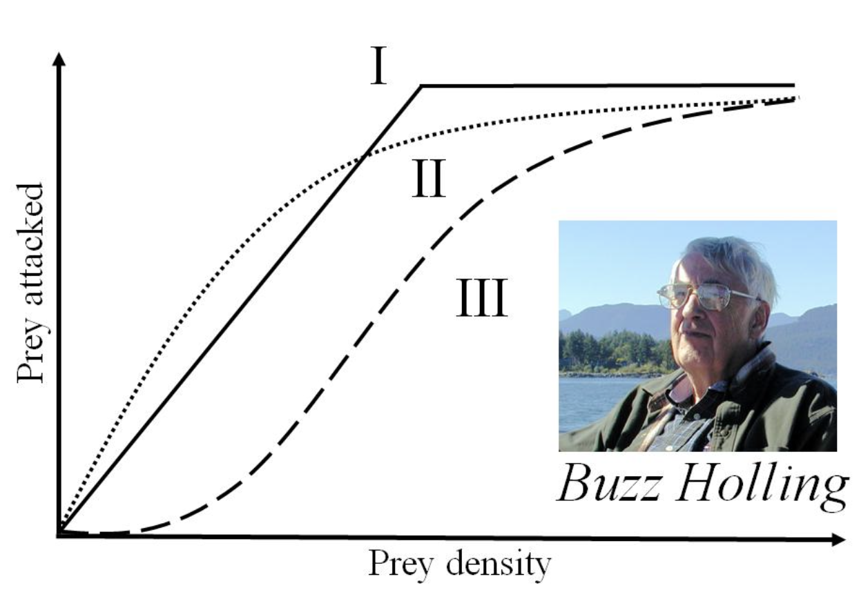
Figure 1. Functional feeding responses as defined by CS Holling.

The Ecosim equations for predicting consumption allow for classic predator-prey functional response types.

• type I if foraging time adjustment is included,
• type II if handling times limit per-capita food-consumption rates, and
• type III if predator rates of search decrease when prey densities are low or prey spend less time foraging when their densities are low

The foraging-arena equations in Ecosim depart from classical functional response predictions in calculating prey densities not as average total biomass in each cell but rather as effective biomass densities in the restricted arenas where foraging typically occurs and where such local densities can be strongly affected by densities of competing predators (ratio-dependence effect). Local depression of available prey biomass can occur whether or not predation affects overall grid-wide prey densities.

Type III switching

Predators are said to “switch” from one prey to another when predator diet proportion of each type changes more rapidly than the relative abundance of that type in the environment. Eating more of something when it becomes abundant does not imply switching, but rather just more frequent encounters with that type. The predator is said to switch if it takes disproportionately more of a prey type as that prey becomes more abundant.

Three mechanisms that can lead to switching patterns in diet composition and prey mortality are represented in Ecosim:

• Apparent switching away from prey that are declining in abundance, due to those prey seeing less intra-specific competition and hence spending less time at risk to predation; this effect occurs for any prey species (and impacts feeding on it by all of its predators) whenever Ecosim>Input>Group info>Feeding time adjust. rate is set >0.
• Apparent switching in Ecospace, caused by fitness-sensitive movement; when Ecospace parameters are set to cause increased (and/or directional) movement from cells where “fitness” (per capita food intake minus instantaneous mortality rate) is lower, predators will appear (for the system as a whole) to switch to more abundant prey, and prey that are declining in abundance will see lower predation rates in the cells where they remain concentrated.
• Explicit changes in Ecosim rates of effective search, representing fine-scale behavioural choices by predators to spend more or less foraging time in the arenas where specific prey is concentrated. In this case, the behavioural choice among arenas is predicted from Ideal Free Distribution (IFD) arguments that predators should allocate foraging time so as to minimize time needed to obtain normal food consumption rates.

In the third of these approaches, the Ecosim rate of effective search a_ij for predator type j on prey type i is modified at each simulation time step in relation to changes in abundance of all prey types, using a “gravity model” approximation for the IFD allocation of predator foraging time among prey-specific foraging arenas. The equation used for this modification is

[latex]a_{ij}(t) = K_{ij}a_{ij}B_i(t)^{P_j} / \sum_{i’} a_{i’j} B_{i’}(t)^{P_j} \tag{1}[/latex]

Here, a_ij is the base rate of effective search calculated from Ecopath and vulnerability exchange parameters, K_ij is a scaling constant that makes the time-specific a_ij(t) equal a_ij when all prey biomasses B_i are at the Ecopath base values, and the “switching power parameter” P_j is a user-supplied (empirical, to be estimated from field data or model fitting) power parameter representing how strongly the predator responds to changes in prey availability (switching power parameter on the Group info form). In particular:

• P_j = 0, no switching
• P_j << 1, prey must become very rare before predator j stops searching for them
• P_j >> 1, predator switches violently when any prey increases or decreases.

P_j is limited to the range [0,2]. While it is derived by pretending that predators must allocate time among mutually exclusive foraging arenas for each of their prey types (a typically unrealistic assumption), it can still be used (with P_j <<1 values) to represent more general ideas about why and how predators switch among prey, e.g., formation and loss of search images for finding them.