1 On modelling and making predictions

Figure 1. Raymond Lindeman (1915-1942).

Food web analyses (and with them ecological networks), as we know them, dates back to the pioneering studies of Raymond Lindeman around 1940 (Figure 1). He studied Cedar Creek Bog in Minnesota and made a detailed model of nutrient cycling expressed as energy flows^[1] (Lindeman 1942). For this, he used thermodynamic principles to evaluate and understand ecosystem functioning, and through this he established the field of trophic dynamics. The study of energy flows and concepts he introduced, such as food chains, food webs, ecological transfer efficiency, and energy pyramids, now provides core elements of community and ecosystem ecology.

Lindeman received a fellowship to work with G. Evelyn Hutchinson at Yale University, managed to publish his PhD studies on Cedar Creek Bog though ill, but unfortunately died soon after, only 27 years old. He was a brilliant mind, and we can only guess how he would have shaped our research world had his days been more numerous.

Lindeman’s studies, however, inspired research for decades to follow.  Most notably, the International Biological Program (IBP), a major international initiative that during 1964-1974 conducted studies of biological productivity in ecosystems throughout the world. Incidentally, this was also where I first participated in ecological research as a first-year student joining the tail end of the study, sampling fish in a lake in Denmark.

Figure 2. Study sites of the International Biological Program (IBP).

The IBP was mainly descriptive in its nature, and had numerous modelling activities including some dynamic ecosystem modelling – a topic to which we return later.  A lasting legacy of the IBP was that it brought focus to ecosystem research. There were also numerous follow-up studies to the IBP. Methodologies had been developed and coordinated through the IBP, and many researchers had been introduced to the field. The time had come for ecosystem research.

Among the follow-up studies was an extensive five-year study conducted around 1980, of the French Frigate Shoals in the Northwestern Hawaiian Islands. Researchers quantified energy flows and biomasses ranging from plankton through to marine mammals, and over the five years gathered an impressive amount of data. Realizing the need to make sense of the mountain of data, NOAA hired a newly graduated oceanographer, Jeff Polovina, to construct an ecosystem model of the French Frigate Shoals.

At this time there were two major activities on ecosystem modelling with a fisheries perspective. Taivo Laevastu and colleagues at the NMFS Alaska Fisheries Science Centre worked on a complex multispecies model of the Bering Sea^[2] (Laevastu and Larkins 1981) while K.P. Andersen and Erik Ursin, at the Charlottenlund Castle, Danish Institute for Fisheries and Marine Research, were constructing an equally complex model of the North Sea^[3]. Polovina evaluated these modelling efforts and realized the impossibility of constructing species-based dynamic models for biologically diverse areas such as a tropical coral reef ecosystem. From the Laevastu model, he adopted the principle of mass-balance, and used this to construct a simple ecological accounting system, which he termed Ecopath.^[4]

Mass-balance here means that energy input has to balance energy output (including storage) for each species (or functional group) that is being modeled. If we can mass-balance one species, we can balance the whole ecosystem. For this, we use information about how much food predators require to compare to how much production is available from their prey. It has to match. And what is important, this adds constraints to the modelling.  Adding constraints is fundamental for all modelling, and is one reason that mass-balance modelling has shown successful. Along with the ease of application this, in 2009 led to the Ecopath modelling approach, (see Figure 3) being recognized by NOAA as one of the ten biggest scientific breakthroughs in the organization’s 200-year history.

Figure 3. The basic Ecopath model creates a snapshot of an ecosystem at a given point in time: who eats who and how much? Mass balance links predator and prey: there has to be enough food for the predators

I have worked with development of the Ecopath with Ecosim (EwE) approach and software for more than three decades, starting off with Daniel Pauly in the Philippines^[5]. Daniel had the idea of merging Polovina’s Ecopath model with ecological network analysis such as developed by Robert Ulanowicz^[6] and others. Finding out how and seeing it through became my PhD work, which was focused on network analysis of trophic interactions based on meta-analysis of aquatic ecosystems.

Figure 4. Eugene P. Odum (1913-2002).

From this work, let me highlight ecosystem development. One of the greatest ecologists of all times, EP Odum (Figure 4) described a set of ecosystem attributes, and how these would change as ecosystems develop^[7]. I quantified most of Odum’s 24 attributes based on some forty Ecopath models, and ranked the models based on maturity^[8]. It worked really well, and since then a number of colleagues have repeated the analysis with the same result. We can rank ecosystems.

It’s typical indicator work. You set a number of criteria, extract the numbers, and out comes a ranking. But what attributes and indicators should we use and how do we obtain the overall ranking? I was really fascinated by this during my PhD: that one could extract a few indicators from food webs and use that to characterize the state of ecosystems.

There are, however, very many indicators and properties in ecological network analysis – you can get the impression that any ecologist doing research in the field in order to be noticed must develop their own way to capture the essence of ecosystems. This, aggravated by very little attempt at evaluating methods and approaches across studies, seems to characterize the field: consensus building has not been an integral part of the development. The big challenge after half a century of ecological network analysis is still to explain what the seemingly endless suite of indicators tells us.

Yet I do not intend to compare network analysis to the “Emperor’s New Clothes” (Figure 5) – though it is a challenge to interpret the many concepts and indicators. I have worked enough with network analysis to see clear patterns, some of which are consistent and rather straightforward to explain, while others are much more elusive. As an example of where I still have unfulfilled expectations of network analysis, let me point to identification of critical species in ecosystems – the canaries in the coal mine, and as part of this, what makes an ecosystem vulnerable to perturbations?

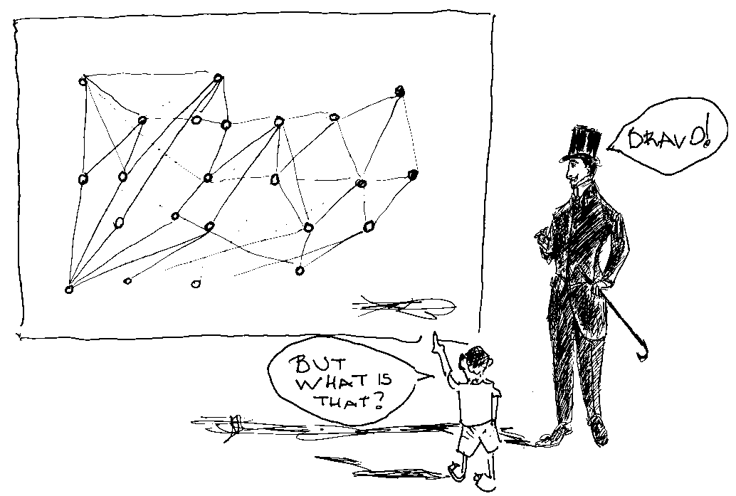
Figure 5. Food web representations can be beautiful, but what do they tell us?

I come to think of the Hitchhiker’s Guide to the Galaxy, especially the third of five volumes in the trilogy^[9]  If you don’t remember it: our planet was really a giant super computer operated by mice. It tolled away for millions of years to answer the biggest and most fundamental question about Life, The Universe and Everything. Eventually the answer came: 42, but by then no one remembered the question. I’ve often been in that situation with network analysis and indicators: It gives the answer, but what was the question? What do the indicators tell us? How do we interpret them? And importantly, can we use this for making prediction?

Making predictions and evaluating “what if” questions remain elusive, however, as ecological network analysis has demonstrated very little predictive capabilities, such as we are craving for in fisheries management. Rather, network analysis tends to be static, almost without exception – it’s the study and interpretation of snapshots such as mentioned earlier.

Dynamic considerations have, however, entered from a different route. There was a productivity sub-group of IBP that focused on modelling, including dynamic modelling of ecosystems. For this, they created a new field in ecology, systems analysis, and recruited a cohort of bright, quantitative young scientists that used the emerging computers to make models and analysis never imagined before.

In essence, what they did was turning the snapshot from the static food web studies into the movie version. And somehow a movie is less open to interpretations than a photo: it adds constraints. But the modelling had problems. All predator-prey modelling is in essence built on Lotka-Volterra dynamics. This means that the consumption by predators is estimated from the product of the number of predators, the number of prey, and a search rate. More predators more consumption; more prey more consumption. Behind this is a thermodynamic principle called mass-action, and this works absolutely fine when mixing reagents and wanting to predict the products. There are, however, problems when using it in ecology.

The systems analysts in the IBP found that their dynamic models were unstable, and commonly experienced cycles and model self-simplification. Cycles are fine when modelling for instance snowshoe hare – lynx interactions in boreal systems^[10], but they are not regular features of more diverse ecosystems. What presented a bigger problem was self-simplification: Lotka-Volterra models are inherently unstable, and it is not possible to maintain ecologically similar groups in models with top-down, mass-action control. The poorer competitors will die out.  This was a problem that marred the modelling of ecosystems, and eventually most or all of the IBP modellers left the field to pursue other avenues.

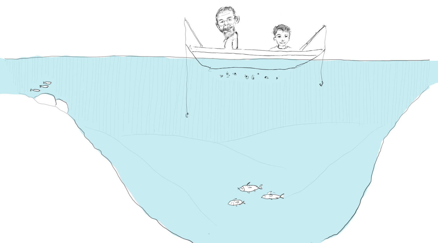
Figure 6. The birth of the foraging arena theory.

One of the bright young fellows in the IBP was my colleague Carl Walters. He had struggled to make ecosystem models behave and given up^[11]. Then one day in the early 90s he was out fishing on a lake in BC with his 9-year-old son, Will. When you fish with Carl you don’t often catch anything, so Will got bored, looked over the side, and saw a lot of nice big Daphnia in the water (Figure 6). He asked: “Why don’t the fish eat them all, Dad?”

Carl went on to give the obvious explanation, one that any fish biologist could have given. “We are fishing for big trout, they are out here in the open and deep part of the lake. The small trout hide along the shore where the big ones don’t come, and it’s the small ones that eat Daphnia. If the small trout come out here, they will be eaten by the big ones”. A simple straightforward explanation, and only afterwards did the profound implications of the reply dawn on him.

The fundamental aspect missing in predator-prey modelling was behavior. Organisms are not randomly moving particles as thermodynamics and mass-action terms tell us. Think of a coral reef with its swarms of planktivores. The small stay close to the safety of the reef, the larger stray a bit further away, but only a safe distance. The moment a roaming piscivore, such as a barracuda, comes patrolling by, they all take cover.

The implication of this is that the prey concentration the piscivores sees is different from the total planktivore abundance, just like the plankton concentration we may measure with nets around the reef is different from what the planktivores actually experience when their foraging is restricted to the immediate safe surroundings of the reef. It takes three to tango: the planktivore (dancer one) restricts its activities in response to the piscivore (dancer two), and this in turn restricts its own access to plankton (dancer three)^[12].

From a modelling perspective, Walters developed an elegant way of adding behavior to the predator-prey modelling through the foraging arena theory^[13]. Organisms change between two behavioral states, being available or unavailable for predation, and including this only calls for adding one additional parameter to the Lotka-Volterra equation, a behavioral exchange coefficient (that relates to carrying capacity).

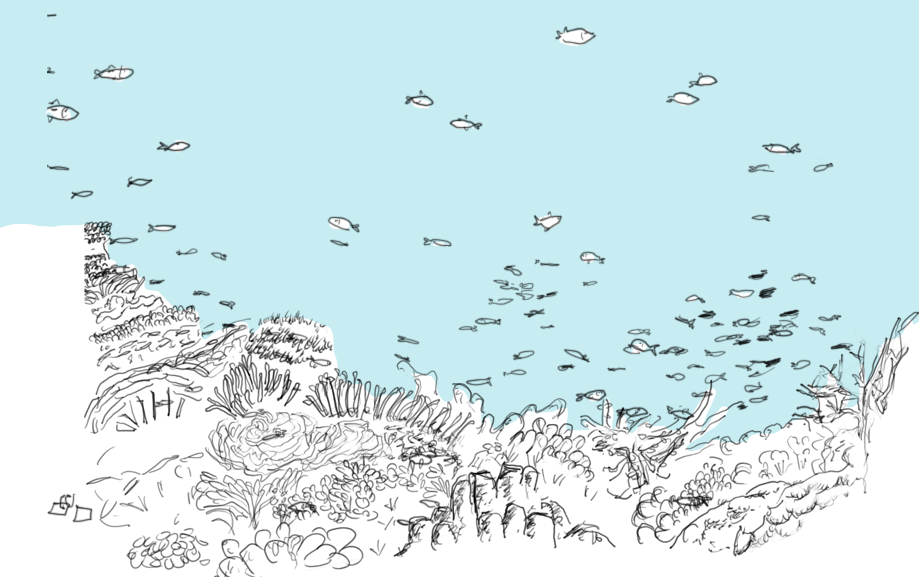Figure 7. Coral reef representation of the foraging arena – the fish are planktivores and stay close to the reef, alert and ready to dive for cover.

One small step of logic, but a giant step for modelling – suddenly the ecosystem models started behaving. Where it had been almost impossible to get models to maintain diversity, incorporation of the foraging arena considerations opened for replicating the known history of ecosystems. This started in earnest a decade ago when fitting ecosystem modelling to time series data started proliferating, and we have since witness a virtual explosion of case studies to the effect that there probable now are more than a hundred of the kind (Figure 8).

Figure 8. Case studies where Ecosim models have been fitted to time series data. The figure was made in 2011, and the number has by now probably tripled or more.

The case studies are based on the Ecosim module of the Ecopath with Ecosim (EwE) approach and software^[14], and we have drawn a number of lessons from them^[15], including what you’ll read in this textbook. As a rule, to explain historic changes in ecosystems we have to consider,

1. Food web effects,
2. Environmental change, and
3. Human impact, (see Figure 9).

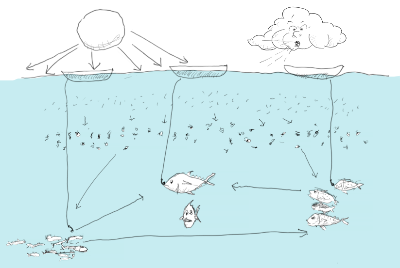Figure 9. Replicating the history of ecosystems calls for inclusion of food web, environmental, and human impact.

An implication of this is that environmental productivity patterns can be identified throughout the food web. There are variable time delays linked to turnover rates and food web constellations, but we can see environmental signals propagate through the food web. We have also seen evidence that environmental productivity can be amplified through the food web.  The biological explanation for this may be that more food results in more excess beyond maintenance, freeing resources to be allocated to growth and reproduction.

Fitting-wise, the models tend to work well for species or groups with strong fisheries impacts, i.e. we generally find good agreements with single-species assessment models. Where there are divergences, they can often be explained from model assumptions related to food web effects. It is also clear that while trends for some species can be explained, there can be others for which the models are unable to offer insight – often because we have no reliable information about what the important drivers of change may be for such species. There is, however, nothing to indicate that such model failures have implications for the overall model fit – here one rotten apple doesn’t spoil the bunch.

Figure 10. The butler did it: humans are the usual suspects when evaluating fish population trends, but ecosystem models can now be used to evaluate the relative contribution of food web, environmental, and human impact.

We see impacts of changes in predator abundance on forage species (prey release), and in some cases the opposite effect; where prey abundance impacts predators. Also, there are cases where fisheries seemingly outcompete predators as increased fishing mortality on a forage species is accompanied by decline in predation mortality^[16] (Walters et al. 2008).

Where ecological networks currently have their biggest potential for contribution in fisheries is for evaluating trade-offs for management. We have reached the point where we with some authority can evaluate trade-offs between alternative uses of fisheries resources^[17].

Summing up, ecosystem models can now replicate historic changes in ecosystems and be used to evaluate the relative impact of fisheries, food web dynamics, and environmental change (Figure 10), and notably use this to evaluate trade-offs. With models that behave well enough to replicate the past, we can start thinking of using them to predict the future, to ask “what-if” questions.

Figure 11. Will there be seafood and healthy oceans for future generations to enjoy?

The key question we have to ask is “will there be seafood and healthy oceans for future generations to enjoy?” (Figure 11). To answer the question, we have to make predictions. There will be uncertainty and unexpected events, but we need to provide  guidelines and options – to ensure that there will be seafood for future generations. What choices must we make for this?

Given that the seafood market is an international one, it is a global question, and we have to tackle the question through modelling scaled accordingly. There is, however, no tradition for global modelling in fisheries, and while the Intergovernmental Panel for Climate Change, IPCC, has done the necessary job on predicting how our physical environment will be impacted by climate change, it is only in recent years that the consequences of climate change on life on earth has gained attention.^[18]

Figure 12. When making predictions, expect the unexpected. The vampire in the basement will bite you.

The Intergovernmental Science-Policy Platform on Biodiversity and Ecosystem Services (IPBES) has taken on this task, and from an aquatic modelling perspective this work is supported by the Fisheries and Marine Ecosystem Model Intercomparison project, Fish-MIP), which works to develop a global ocean-modelling framework that incorporates modelling of the physical environment, of lower and higher trophic levels, and of human activities including governance. Fish-MIP provides a framework with alternative modelling components in order to consider uncertainty through an ensemble approach, following the lead for how the IPCC has tackled global environmental modelling.

Uncertainty indeed has to be a major factor in making predictions. While ecosystem models now offer some predictive capabilities for evaluating major human impacts and making predictions, we cannot make beautiful orchestrated symphonies or detailed predictions, and we will never be able to do that for complex ecosystems. There are notably two factors that prevent this. One is Walter’s “vampires in the basement” (Figure 12), the other is incomplete knowledge of how systems will react to management interventions.

We must expect the unexpected; there will be events we cannot predict. Invasive species is a case in point, and more generally, behavioral responses in ecosystems are no more predictive than they are for human systems. Let me illustrate with an example; seals have been increasing in the Strait of Georgia since culling ceased in the 1970s. For about 30 years thereafter, mammal-eating transient killer whales were rarely observed in the Strait. Then one summer, a small pod came in and found plenty of prey – the next summer the whale watching boats counted a hundred transient killer whales coming in, and transients have been regular visitors since then. From a modelling perspective, such behavioural events are unpredictable, and they have repercussions through the ecosystems.

Figure 13. Monitor, experiment, and adapt. The fundamental aspects of adaptive management rely on modelling as the guiding factor.

There is also considerable uncertainty about how ecosystems will react to many management interventions, especially where our knowledge about drivers and impact is very incomplete. Our best option wherever this is the case is represented by adaptive management with carefully planned monitoring, experimentation, and adaptation^[19]. Modelling is an integral part of this, needed to guide the entire process and limit the risk of making bad, preventable mistakes.

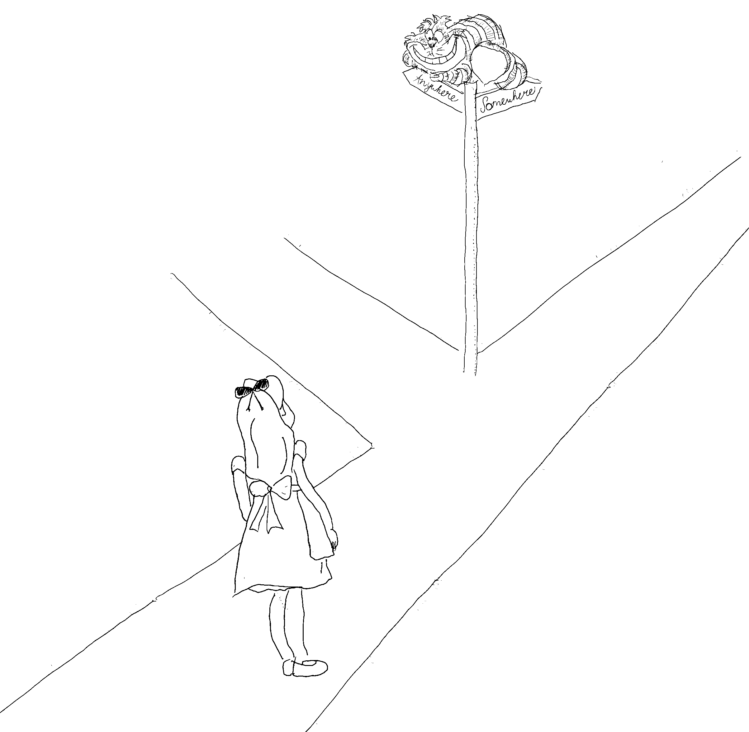
Figure 14. Alice: “Would you tell me, please, which way I ought to go from here?” 
Cheshire Cat: “That depends a good deal on where you want to get to”. Policy makers need to set clear objectives for management, and scientists need to evaluate alternative options for managers.

So, though we cannot make detailed predictions for how ecosystems will develop, we as a society need to carefully choose what direction to take and we need to avoid the preventable mistakes.  For this, it is crucial that fisheries policy makers and managers set clear objectives for management, and that fishery scientists in turn define and evaluate alternative policy options (Figure 14). We need to manage our ecosystems with a strong commitment to moving in a sustainable direction if there indeed is to be seafood and healthy oceans for future generations to enjoy.