17 Predicting consumption

This is what Ecosim (and all other dynamic ecosystem models) really is about. If the number of consumers change over time, how much do they eat? How does consumption change with population density?

All ecosystem models predict consumption (Q_ij) changes based on a variant of Lotka-Volterra dynamics (see chapter), including Ecosim which uses simple Lotka-Volterra or “mass action” assumptions for prediction of consumption rates. But importantly, the assumption is modified to consider “foraging arena” properties so that the flow rates depend on abundance of vulnerable prey rather than total prey abundance. In the foraging arena model structure, prey can be in states that are or are not vulnerable to predation, for instance by hiding, (e.g., in crevices in reefs, inside a school, where predators don’t go) when not feeding, and only being subject to predation when having left their shelter to feed. (see chapter).

In the original Ecosim formulations^{[1]  [2]}) the foraging arena consumption rate for a given predator i feeding on a prey j was predicted as,

[latex]Q_{ij}=\frac{a_{ij} \ v_{ij} \ B_i \ B_j}{2v_{ij}+a_{ij} \ B_j}\tag{1}[/latex]

where, a_ij is the effective search rate for predator j feeding on a prey i, v_ij base vulnerability expressing the rate with which prey move between being vulnerable and not vulnerable, B_i prey biomass, and B_j predator abundance (for multi-stanza groups, B_j in this calculation is replaced by an estimate of the area swept by organisms of varying sizes, summed over ages within each stanza).

The model as implemented implies that “top-down vs. bottom-up” control is in fact a continuum, where low v’s implies bottom-up and high v’s top-down control.

Experience with Ecosim has led to a more elaborate expression to describe how consumption may vary with a variety of factors:

[latex]Q_{ij}=\frac{v_{ij} \ a_{ij} \ B_i \ B_j \ T_i \ T_j \ S_{ij} M_{ij}/D_j }{v_{ij}+v_{ij} \ T_i \ M_{ij}+a_{ij} \ M_{ij} \ B_j \ S_{ij} \ T_j/D_j/A} \cdot f(Env_t)\tag{2}[/latex]

where, T_i represents prey relative feeding time, T_j predator relative feeding time, S_ij user-defined seasonal or long term forcing effects, M_ij mediation forcing effects, A is foraging arena size, f(Env_t) is an environmental response function that impacting the size of the foraging arena to account for external drivers, which may change over time^[3], and D_j represents effects of handling time as a limit to consumption rate (1/D_j is proportion of time spent feeding):

[latex]D_j={1+h_j\sum_k a_{kj} V_k T_k M_{kj}}\tag{3}[/latex]

where h_j is the predator handling time and V_k is the vulnerable density of prey type k to predator j (V_k is estimated numerically in the Ecosim code).

The food consumption prediction relationship in the second equation above contains two parameters that directly influence the time spent feeding and the predation risk that feeding may entail: a_ij and v’_ij. To model possible linked changes in these parameters with changes in food availability over time (t) as measured by per biomass food intake rate c_i,t = Q_i,t / B_i,t we need to specify how changes in c_i,t will influence at least relative time spent foraging.

Denoting the relative time spent foraging as T_i,t, measured such that the rate of effective search during any model time step t can be predicted as a_ji,t = T_i,t a_ij for each prey type i that j eats, we may (optionally) assume that time spent vulnerable to predation, as measured by v’_ij for all predators j on i, is inversely related to T_i,t, i.e., v’_ij,t = v’_ij / T_i,t. An alternative structure that gives similar results is to leave the a_ij constant, while varying the v_ij by setting v_ij,t = T_j,t · v_ij in the numerator of Eq. 2 and v_ij,t = T_i,t · v_ij in the denominator.

For convenience in estimating the a_ij and v’_ij parameters, we scale T_i,t so that T_i,0 = 1, and v’_ij= v_ij. Using these scaling conventions, the key issue then becomes how to functionally relate T_i,t to food intake rate c_i,t so as to represent the hypothesis that animals with lots of food available will simply spend less time foraging, rather than increase food intake rates.

In Ecosim, a simple functional form for T_i,t is implemented that will result in near constant feeding rates, but changing time at risk to predation, in situations where rate of effective search a_ij is the main factor limiting food consumption rather than prey behaviour as measured by v_ji. This is implemented in form of the relationship,

[latex]T_{i,t}=T_{i,t-1 }(1-α+α\frac{Q_{opt,i,t}}{Q_{i,t-1}}) \tag{5}[/latex]

where, a is a feeding time adjustment rate [0, 1]and Q_opt is the Ecopath base consumption rate per biomass (QB) for group j .  This calculation is subject to a user-defined maximum relative foraging time for each predator, and the result of that upper limit is for the predator functional response to be approximately the Holling Type I (rectilinear, see Holling functional response chapter) form with steepness proportional to the maximum relative foraging time.

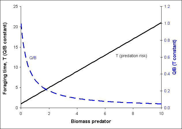
The relationship between foraging time, consumption and predator biomass (when adjustment rate a is assumed nonzero) is illustrated in Figure 1.

Figure 1. Relationship between relative foraging time (T), Q/B and predator biomass. If Q/B is held constant the foraging time (and hence predation risk) is a linear function of the predator biomass (solid line). If T is held constant the Q/B will decrease asymptotically with predator biomass (stippled line). The predation risk is assumed proportional to the relative foraging time.