Tutorial: Spatial model of Anchovy Bay
Learning Objectives
- Introduction to basic Ecospace operations
- Introduction to the habitat capacity model of Ecospace
Getting started
Open the Anchovy Bay model that we created in a previous tutorial (or download it). Load the time series that we previously added to Ecosim (or check the Ecosim time series tutorial to get the time series – link to csv file). Open Ecospace and create a new scenario (you decide what to call it).
Go to Ecospace > Input > Ecospace parameters tab: If you loaded the time series then the Run time on the tab is likely to be 41 years, and number of time steps is 12. Notice that Ecospace can use variable time steps, but fine to leave this at 12 (monthly) time steps per year.
Next task is to create the spatial map that we will use for the tutorial: Click Ecospace > Input > Maps in the Navigator. At the top of the right-hand side panel, click Edit basemap. Set Number of rows to 20, and Number of cols (columns) to 20. This gives us 20 x 20 = 400 cells to work with. More would give us a prettier picture, take longer time to run, and not necessarily give us different results. Set Cell length to 5.65 km. Click OK. EwE will save and close the form.
Select Input > Maps again, and click Depth at the right-hand side panel. Now click the icon to the right of Depth. This will open a form that will allow you to: Edit Layer ‘Depth’. Click the Data tab, and you will get a spreadsheet.
Now download and open the spreadsheet Spatial Anchovy Bay.xlsx, and on the first tab (Depth), highlight the values (including row and col numbers), the press Ctrl + C (for copy).
Go back to Ecospace, click the top left cell in the depth data spreadsheet, and press Ctrl + V (for paste). You should now have the depth map for Anchovy Bay.
Habitat capacity model
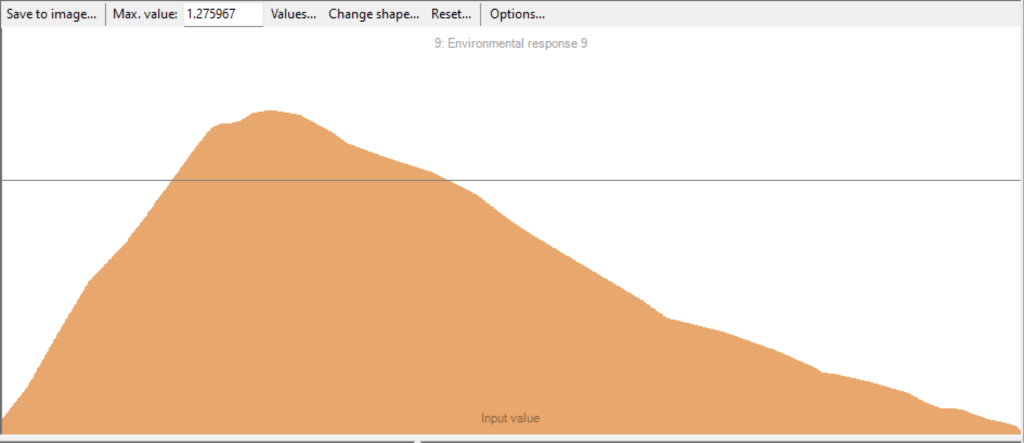
Figure 1. Example of a hand-drawn response function. Ecospace will rescale the Y-axis, so the shape matters, but not the amplitude.
Next, we want to start parameterizing the habitat capacity model. Here, we’ll illustrate this with a simple example (before loading a version of the model with more layers). Click Ecospace > Input > Ecospace environmental responses. Click Add on the lower center panel in order to add a response curve. For now, think of this shape as representing the depth distribution of a species, e.g., for cod. We can read in such shapes, but for now just get by with a sketched shape. So draw a shape, for instance with a low value at low X, then increasing to a max at 1/3 of the max X-value and then gradually declining to 0 again. (Maybe somewhat as in Figure 1).
First, we need to define the X-axis, (Ecospace > Input > Ecospace environmental responses > Define environmental response). Set X-min and X-max above the right-hand side panel. Leave X-min at 0. Set X-max to, e.g., 400 m (just to try it). Click OK, and X-axis on the Driver histogram & response function plot below should update.
Now we have to assign the functional response above to cod. Go to Ecospace > Input > Ecospace environmental responses > Group capacity model, and select Use environmental responses for all groups. (Just click the row header, and it will select all, then change the box in the top right to True). It is OK to have both Use habitat and Use environmental responses selected, (but we won’t be using the habitats here, so you can also uncheck the Use habitat – though it makes no difference when there are no habitats defined).
Next, go to Ecospace > Input > Ecospace environmental responses > Apply foraging response. In the spreadsheet, click the cell under Depth for Cod. In the left panel, click the shape you made, click the green arrow to the right, OK to assign this shape to cod. There will be a histogram of depth values up in the panel to the right. This histogram is just for your reference. Now we are to Click OK to exit the form.
Now it’s time to run Ecospace. Go to Ecospace > Output > Run Ecospace, and click the Run Ecospace button at the bottom-left of the center panel. By default, Ecospace will show you a time plot, but you can see spatial maps, it you select the Map tab above the time plot. On the small distribution maps that appears, you should see that cod have a distribution that is impacted by the functional response you defined.
Explore the Ecospace model a bit.
Anchovy Bay Spatial
Next, let’s read in a version of the model that has more data. Download the file Anchovy Bay Spatial.ewemdb.zip from this link. It has a new version of the Anchovy Bay database. Unzip and open the database in EwE.
Go to Ecospace > Input > Ecospace environmental responses, and explore the additional shapes (see Figure 2).
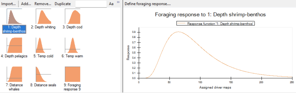
Figure 2. Nine environmental response function plots (left panel). Each of these figures describes a plot as indicated in the right panel. This example shows the depth foraging response for shrimp and benthos, which are assumed to show a log-normal like distribution ranging from 10 to 250 meters depth with a peak around 70 meters.
On the next tab, Ecospace > Input > Ecospace environmental responses > Apply foraging arena shapes, you can find an example of how to allocate shapes for the model groups (Table 1).
Check if the model you use has environmental drivers defined. On the Ecospace > Input > Maps page, click the pen icon by Environmental drivers in the right-hand listing, and define the input driver maps here. For this Anchovy Bay tutorial that would be Depth (which already is there), temperature and distance from coast.
Table 1. Applied environmental response function shapes.
| Group no | Group name | Depth | Temperature | Distance from coast |
| 1 | Whales | 3: Depth cod | 7: Distance whales | |
| 2 | Seals | 2: Depth whiting | 8: Distance seals | |
| 3 | Cod | 3: Depth cod | 5: Temp cold | |
| 4 | Whiting | 2: Depth whiting | 6: Temp warm | |
| 5 | Mackerel | 4: Depth pelagics | 5: Temp cold | |
| 6 | Anchovy | 4: Depth pelagics | 6: Temp warm | |
| 7 | Shrimp | 1: Depth shrimp-benthos | ||
| 8 | Benthos | 1: Depth shrimp-benthos | ||
| 9 | Zooplankton | |||
| 10 | Phytoplankton | |||
| 11 | Detritus |
The habitat based foraging arena shapes are used for each functional group to calculate how much foraging arena there is in each spatial cell in the model. As such it replaces or supplements the habitats that were used in previous versions of Ecospace – which either were good or bad for the individual groups, see the Habitat capacity chapter.
The original type of defined habitats can still be included in Ecospace. This is for (1) compatibility with existing Ecospace models, (2) for use to restrict groups to specified habitat types, and (3) for potential use to allocate effort for fishing fleets. This is illustrated in the present tutorial, see Ecospace > Input > Maps, where you under Habitats in the right-hand side panel, can find four habitats, Coastal, Sand, Rocky, and Deep. These habitats are used on the Ecospace > Input > Ecospace Fishery tab to allocate fleets to habitats; e.g., the trawlers are not able (or allowed) to operate in cells with rocky bottom.
Note that explicit habitats can occupy a fraction of a cell. See for instance the Rocky habitat. Click on the Icon to the right of Rocky, which brings up the: Edit layers ‘Rocky’. (This is where you can change the map icon for the habitat). Here, click Data on the top left, and you can see that there are rocky reefs in fractions of some habitats.
Run and explore the model.
Media Attributions
- Ecospace > Input > Ecospace environmental responses > Add form
