Tutorial: Spatial optimization
Learning Objectives
- Obtain experience with how to set up Ecospace for optimization as part of marine spatial planning
We use the spatial ecosystem model of Anchovy Bay that we have worked with in a number of previous tutorials. The purpose of this exercise is to evaluate alternative placements of marine protected areas, and evaluate which gives most protection at the least cost. The EwE spatial optimization routine is described by Christensen et al. (2009)[1]
Importance layers for conservation
Anchovy Bay has a number of species and habitats that are of conservation concern, including,
- a threatened dugong population that is protected and occurring in areas with human activities that may impact the population recovery.
- a bird nesting area where ships may disturb breeding birds and fisheries deplete resources close to the breeding area,
- two estuaries that are important as fish rearing areas and for biodiversity, and
- an extensive hard bottom area, which among other is home to a rare, endangered and protected species: Charcharodon endangerous.
The groups of conservation concern are not included in the Anchovy Bay model, (which is focused on commercially important fish species, their prey groups and competitors along with socio-economic aspects), so how do we go about modelling their protection? The spatial optimization module of EwE is designed with that in mind. The first task is to obtain distribution maps for the groups of concern, and read those into Ecospace. Subsequently, we will define an objective function based on economic, social and ecological factors, and search for a protection scheme that will optimize conservation concern at the least possible cost (as defined through the objective function).
For the conservation layers, we need raster maps, i.e. spreadsheet-like maps with rows and columns quantifying for each cell how much there is of the area of concern. For instance, expressing how often dugongs are observed in each spatial cell.
For Anchovy Bay, we have such distribution maps for the four groups as concern (Figure 1), and you can download the file Importance layers.zip from this link. The file has four CSV files, one for each of the four conservation or importance layers.
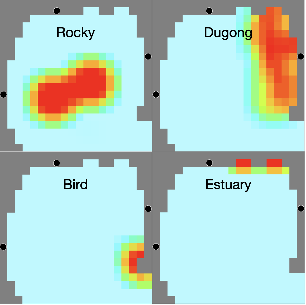
Figure 1. Importance layers imported from CSV files to Ecospace > Input > Maps > Importance.
 Figure 2. Adding importance layers (click the pen to the right of Importance)
Use a version of your Anchovy model for which you have already defined the spatial distribution of the Ecopath groups. You can download a zipped version of the Anchovy Bay spatial database from here, if required. Open the Anchovy Bay spatial, and the Ecospace scenario with spatial distributions. Then go to Ecospace > Input > Maps and in the right-side column, click the pencil to the right of where it says Importance (0) (Figure 2). [If it says Importance (4), you can skip this step, the importance layers have already been defined]. Now add four layers, and name them: Rocky bottom, Dugong feeding, Bird nesting, and Estuary. Click OK.
In the right-side column, you should now have the four importance layers. Double-click where it says Rocky bottom, and an Edit layer form should pop-up. Here you can either cut-and-paste the content from the Rocky bottom.csv file (that were in the Importance layers.zip file), or you can select Import > from CSV… and import the csv file directly. Do the same for the three other importance layers, and check that you have density maps for each.
Note that if you click on the name of an importance layer, you can edit the given importance layer with the tools in the lower part of the right-hand side column – at the bottom section named Importance. This is especially useful to quickly develop and evaluate hypotheses – you can do that before you have actual distribution maps, and get an idea of what’s important and what’s not. The philosophy is: model first, data later.
Now go back to Ecospace > Input > Maps > Importance (4) and click the pen to the right. In the form, the second column will give the weight of each distribution layer with a default value of 1. Using the default values mean that later when the spatial optimization routine selects cells for protection, cells from each of the four distributions are equally likely to be included, irrespective of how many cells there are in each layer. Hence, a given cell in a layer that has only a few cells (e.g., Estuary) is more likely to be protected than a given cell in a layer with many cells (e.g., Hard bottom).
Two final checks before we go to the spatial optimization routine,
- Check if you have a marine protected area (MPA) defined. On Ecospace > Input > Ecospace fishery > Marine Protected Areas, you can check if you already have any MPAs defined. If not, click Define MPAs at the top row, and add an MPA. OK. On the form, you can define which months the MPA is closed – leave it at closed all months. Further, on Ecospace > Input > Ecospace fishery > MPA enforcement, you can define if individual fleets are allowed to operate in an MPA or not. The default is that no fleets are allowed to work in any MPAs, leave it at that.
- Check the dispersal rates in your model, Ecospace > Input > Dispersal. Set Base dispersal rates to 10 km year-1 (click the column title Base dispersal rate, and enter 10 in the Apply box). This highly unrealistic setting will make the MPAs more efficient at building up biomass, and is only used to better illustrate how the optimization routine functions.
Objective function
The spatial optimization module is at Ecospace > Tools > Spatial optimizations. On the rather complex form that pops up, you can define and run the optimizations. At the top, Search type, select Importance layer. The next steps are all on the Parameterization tab.
First, set Start year to 30. With this the optimization routine will first do a run of Ecospace, and store the state at Year 30. The optimizations will then only do each model run from year 30 to 41. This is to speed up things in this tutorial, you will need to evaluate how long time it takes for MPA effects to be significant in a real application before deciding. Also set the Base year to 30, which tells Ecospace that the economic and social factors are for that year. In the first column, check that the MPA drop-down list is set to the MPA you want to optimize for (in case you have several MPAs defined).
In the next column, you can set how much of the area that should be closed (in percentage of the number of water cells, i.e. not counting land cells). For now, leave this at the default 20%. Also, set the number of iterations to 20 – in a real application you would use many more, hundreds or more likely, thousands.
Next, we define the objective function, this is done in the left-most table in the next row. The objective function includes the elements from the policy optimization plus a few add-ons,
- Net economic value, i.e. the profit made by the fishing fleet (or in the overall fishing sector if the value chain is defined and used)
- Social value (employment), defined based on the job/catch value from the second table (or through the value chain)
- Mandated rebuilding, can be used to force rebuilding if target values are entered in the third table, first column
- Ecosystem structure is an ecological measure based on one of EP Odum’s maturity indicators: maximizing the average longevity in an ecosystem (which characterizes mature stable ecosystems). We capture this with the inverse P/B, i.e. B/P (unit: year), which expresses the average longevity of a group. The default values are B/P from the Ecopath base model, excluding fast turnovers (e.g., shrimp and zooplankton), and you can consider, which groups you think it’s reasonable to include. For now, you can just leave it at the default values.
- Biodiversity optimizes by default for the Shannon index, used to express how uniform the biomass distribution is across the functional groups in the model, assuming that it ecologically is more optimal to have the biomass more distributed rather than concentrated on a few groups.
- Boundary weight is used to capture how continuous the MPA network is. The index is calculated as the length of the boundary between cells protected and not protected divided by the total MPA area. For instance, one cell in an MPA will have a boundary weight of 0.25 (area = 1, boundary = 4), whereas two adjacent cells will have a boundary weight of 0.33 (area = 2, boundary = 6). A 2 x 2 cluster of MPA cells will have a boundary weight of 0.5.
For this tutorial, set the Net economic value to 1, the Social value to 1, and the Boundary weight to 1.
In the third table, the Max fishing mortality can be set to avoid that groups are fished unsustainably by entering the maximum acceptable fishing mortality for groups of concern.
Model runs
That’s it, ready to run. Press the run button, and you can select the Map tab to see what it is doing. Once completed, you can select results from the runs with the highest value of the objective function at the bottom of the form. The default is the 10% of the runs with the highest value, that means the two best runs when there’s only 20 runs. In a real application, you may have thousands of runs, and you would select a lower percentage of the runs, perhaps the best 1%.
In the right-most panel, you can select the Best count layer, and it will show how many times each cell was included in the best runs. This is indicated by the heat map, and you can see the count if you hover over a cell with the mouse pointer.
If you want to, you can click Convert to MPA, and the best cells will be transferred to the MPA layer in Ecospace. Do that, and check it out (Ecospace > Input > Maps, MPA layer), it will be a pretty spotty map with so few runs, but it serves to illustrate the functionality.
Try to change the weights for the importance layers, (available on Ecospace > Tools > Spatial optimizations > Importance layers tab above the map lot). For instance to set the weight for Hard bottom to 1, and the rest to 0. This should lead to more contagious cell selection. Go back to the Spatial optimization module, and try running again.
Play! That’s how we all learn and it’s much more funner than school.
Media Attributions
- Ecospace > Input > Maps > Importance
- Ecospace > Input > Maps, adding Importance layers
- Christensen, V., Z. Ferdaña, J. Steenbeek. 2009. Spatial optimization of protected area placement incorporating ecological, social and economic criteria. Ecological Modelling 220:2583-2593 ↵
