23 Dynamic instability and multiple stable states

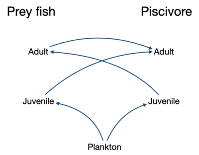
Figure 1. Complex ontogenetic feeding relationship impacting predator-prey balance.  A predator may cultivate the environment for its juveniles by feeding on a prey that competes and perhaps prey on its own juveniles.  If the predator abundance is reduced, e.g., by fishing, the prey abundance may increase, potentially making it difficult for the predator to rebound. In models we often see alternate stable states occurring when a prey species feed on the young stages of its predators.   

Dynamic instability in Ecosim and Ecospace

We commonly see several types of dynamic instability following small perturbations in fishing mortality rates (to get away from initial Ecopath equilibrium):

• Predator-prey cycles and related multi-trophic level patterns;
• System simplification (loss of biomass pools due to competition/predation effects);

• Stock-recruitment instabilities (cyclic or erratic changes in recruitment and stock size for split pool groups);
• Numerical “chatter” in time solutions (mainly in Ecospace).

Such patterns are not particularly common in fisheries time series, so unless you have data to support a cyclic prediction, it’s probably reasonable to adjust the model parameters to get rid of it.

Predator-prey and simplification effects can usually be eliminated by reducing the predation vulnerability multipliers (Ecosim > Input > Vulnerability multipliers form, set values to 4 or less).

We know of at least four common mechanisms that can decrease the vulnerability multipliers so as to create stabilizing and the appearance of “ratio-dependent” or “bottom-up” control of consumption rates:

• Risk-sensitive prey behaviours: Prey may spend only a small proportion of their time in foraging arenas where they are subject to predation risk, otherwise taking refuge in schools, deep water, littoral refuge sites, etc.
• Risk-sensitive predator behaviours (the “three to tango” argument): Especially if the predator is a small fish, it may severely restrict its own range relative to the range occupied by the prey, so that only a small proportion of the prey move or are mixed into the habitats used by it per unit time. In other words, its predators may drive it to behave in ways that make its own prey less vulnerable to it.
• Size-dependent graduation effects: Typically a prey pool represents an aggregate of different prey sizes, and a predator can take only some limited range of sizes, limited vulnerability can represent a process of prey graduation into and out of the vulnerable size range due to growth. Size effects may of course be associated with distribution (predator-prey spatial overlap) shifts as well.
• Passive, differential spatial depletion effects: Even if neither prey or predator shows active behaviours that create foraging arena patches, any physical or behavioural processes that create spatial variation in encounters between predator and prey will lead to local depletion of prey in high-risk areas and concentrations of prey in partial predation “refuges” represented by low-risk areas. “Flow” between low and high-risk areas (v_ij) is then created by any processes that move organisms.

These mechanisms are so ubiquitous that any reader with aquatic natural history experience might wonder why anyone would ever assume a mass-action, random encounter model (high vulnerability multipliers (e.g., 100) in the Ecosim > Input > Vulnerability multipliers form) in the first place.

Methods for dealing with stock-recruitment instability are discussed in the help section on using Ecosim to study compensation. Generally, the simplest solutions are to check (and reduce if needed) cannibalism rates, set higher foraging time adjustment rates (Ecosim > Input > Group info form) for juvenile pools and reduce vulnerabilities of prey to juvenile fishes (Ecosim > Input > Vulnerability multipliers form).

Numerical instabilities (chatter, oscillations of growing amplitude) occur mainly in Ecospace. They are avoided in Ecosim by only doing time dynamic integration of change for pools that can change relatively slowly. In Ecospace, the only remedy for chatter is to reduce the prediction time step (from 12/year default value, sometimes very low values such as 0.05 year are required for stability). In extreme cases, it might be necessary to “fool” Ecosim and Ecospace by implicitly moving to a shorter time step for all dynamics, which you can do by dividing every Ecopath input time rate (P/B, Q/B) with the same factor.

Multiple stable states

With careful parameter choices, Ecosim can also represent Holling’s resilience concept of multiple stable states. In particular, so-called “cultivation-depensation”^[1] or “trophic triangle” effects can lead to stable states dominated by large or small species, with the initial Ecosim equilibrium being an unstable or saddle-point between these states, (see Figure 1).  For example, suppose a dominant large species like cod is fished down, and that one or more of its prey species then increase.  If the prey species, then consume or compete with juveniles of the cod, cod  juvenile survival rates may be reduced enough to cause the cod to continue to collapse, leading to a stable equilibrium dominated by the smaller species.  As a historical note, the very first Ecosim model was developed by Alida Bundy for Manila Bay in the Philippines.  That model exhibited two stable states for two competing groups of small Leiognathid fishes, with small perturbations from the initial Ecosim state lead to dominance by one or other of the two groups.