7.4 Coupled Equilibria

Vishakha Monga; Paul Flowers; Klaus Theopold; William R. Robinson; Richard Langley

7.4 Coupled Equilibria

Learning Objectives

By the end of this section, you will be able to:

Describe examples of systems involving two (or more) coupled chemical equilibria
Calculate reactant and product concentrations for coupled equilibrium systems

As discussed in preceding chapters on equilibrium, coupled equilibria involve two or more separate chemical reactions that share one or more reactants or products. This section of this chapter will address solubility equilibria coupled with acid-base and complex-formation reactions.

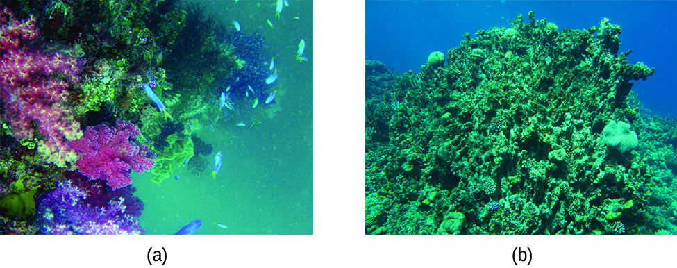
An environmentally relevant example illustrating the coupling of solubility and acid-base equilibria is the impact of ocean acidification on the health of the ocean’s coral reefs. These reefs are built upon skeletons of sparingly soluble calcium carbonate excreted by colonies of corals (small marine invertebrates). The relevant dissolution equilibrium is:

${\text{CaCO}}_{3}\left(s\right)\phantom{\rule{0.2em}{0ex}}$\rightleftharpoons$\phantom{\rule{0.2em}{0ex}}{\text{Ca}}^{2+}\left(aq\right)\phantom{\rule{0.2em}{0ex}}+\phantom{\rule{0.2em}{0ex}}{\text{CO}}_{3}{}^{2-\phantom{\rule{0.2em}{0ex}}}\left(aq\right)\phantom{\rule{5em}{0ex}}{K}_{\text{sp}}\phantom{\rule{0.2em}{0ex}}=\phantom{\rule{0.2em}{0ex}}8.7\phantom{\rule{0.2em}{0ex}}\times\phantom{\rule{0.2em}{0ex}}{10}^{-9}$

Rising concentrations of atmospheric carbon dioxide contribute to an increased acidity of ocean waters due to the dissolution, hydrolysis, and acid ionization of carbon dioxide:

${\text{CO}}_{2}\left(g\right)\phantom{\rule{0.2em}{0ex}}$\rightleftharpoons$\phantom{\rule{0.2em}{0ex}}{\text{CO}}_{2}\left(aq\right)$

${\text{CO}}_{2}\left(aq\right)\phantom{\rule{0.2em}{0ex}}+\phantom{\rule{0.2em}{0ex}}{\text{H}}_{2}\text{O}\left(l\right)\phantom{\rule{0.2em}{0ex}}$\rightleftharpoons$\phantom{\rule{0.2em}{0ex}}{\text{H}}_{2}{\text{CO}}_{3}\left(aq\right)$

$\begin{array}{ccc}\hfill {\text{H}}_{2}{\text{CO}}_{3}\left(aq\right) \phantom{\rule{0.2em}{0ex}}+\phantom{\rule{0.2em}{0ex}}{\text{H}}_{2}\text{O}\left(l\right)\phantom{\rule{0.2em}{0ex}}$\rightleftharpoons$\phantom{\rule{0.2em}{0ex}}{\text{HCO}}_{3}{}^{-}\phantom{\rule{0.2em}{0ex}}\left(aq\right)\phantom{\rule{0.2em}{0ex}}+\phantom{\rule{0.2em}{0ex}}{\text{H}}_{3}{\text{O}}^{+}\phantom{\rule{0.2em}{0ex}}\left(aq\right) \hfill & & \hfill {K}_{\text{a}1}\phantom{\rule{0.2em}{0ex}}=\phantom{\rule{0.2em}{0ex}}4.3\phantom{\rule{0.2em}{0ex}}\times\phantom{\rule{0.2em}{0ex}}{10}^{-7}\hfill \end{array}$

$\begin{array}{ccc}\hfill {\text{HCO}}_{3}{}^{-}\phantom{\rule{0.2em}{0ex}}\left(aq\right)\phantom{\rule{0.2em}{0ex}}+\phantom{\rule{0.2em}{0ex}}{\text{H}}_{2}\text{O}\left(l\right)\phantom{\rule{0.2em}{0ex}}$\rightleftharpoons$\phantom{\rule{0.2em}{0ex}}{\text{CO}}_{3}{}^{2-\phantom{\rule{0.2em}{0ex}}}\phantom{\rule{0.2em}{0ex}}\left(aq\right)\phantom{\rule{0.2em}{0ex}}+\phantom{\rule{0.2em}{0ex}}{\text{H}}_{3}{\text{O}}^{+}\phantom{\rule{0.2em}{0ex}}\left(aq\right)\hfill & & \hfill {K}_{\text{a}2 }\phantom{\rule{0.2em}{0ex}}=\phantom{\rule{0.2em}{0ex}}4.7\phantom{\rule{0.2em}{0ex}}\times\phantom{\rule{0.2em}{0ex}}{10}^{-11}\hfill \end{array}$

Inspection of these equilibria shows the carbonate ion is involved in the calcium carbonate dissolution and the acid hydrolysis of bicarbonate ion. Combining the dissolution equation with the reverse of the acid hydrolysis equation yields:

$\begin{array}{ccc}\hfill {\text{CaCO}}_{3}\left(s\right)\phantom{\rule{0.2em}{0ex}}+\phantom{\rule{0.2em}{0ex}}{\text{H}}_{3}{\text{O}}^{+}\left(aq\right)\phantom{\rule{0.2em}{0ex}}$\rightleftharpoons$\phantom{\rule{0.2em}{0ex}}{\text{Ca}}^{2+}\left(aq\right)\phantom{\rule{0.2em}{0ex}}+\phantom{\rule{0.2em}{0ex}}{\text{HCO}}_{3}{}^{-}\phantom{\rule{0.2em}{0ex}}\left(aq\right)\phantom{\rule{0.2em}{0ex}}+\phantom{\rule{0.2em}{0ex}}{\text{H}}_{2}\text{O}\left(l\right) \hfill & & \hfill K\phantom{\rule{0.2em}{0ex}}=\phantom{\rule{0.2em}{0ex}}{K}_{\text{sp}}\phantom{\rule{0.2em}{0ex}}\text{/}\phantom{\rule{0.2em}{0ex}}{K}_{\text{a}2}\phantom{\rule{0.2em}{0ex}}=\phantom{\rule{0.2em}{0ex}}180\hfill \end{array}$

The equilibrium constant for this net reaction is much greater than the K_sp for calcium carbonate, indicating its solubility is markedly increased in acidic solutions. As rising carbon dioxide levels in the atmosphere increase the acidity of ocean waters, the calcium carbonate skeletons of coral reefs become more prone to dissolution and subsequently less healthy (Figure 7.4.1).

This figure contains two photographs of coral reefs. In a, a colorful reef that includes hues of purple and pink corals is shown in blue green water with fish swimming in the background. In b, grey-green mossy looking coral is shown in a blue aquatic environment. This photo does not have the colorful appearance or fish that were shown in figure a. — Figure 7.4.1 – Healthy coral reefs (a) support a dense and diverse array of sea life across the ocean food chain. But when coral are unable to adequately build and maintain their calcium carbonate skeletons because of excess ocean acidification, the unhealthy reef (b) is only capable of hosting a small fraction of the species as before, and the local food chain starts to collapse. (credit a: modification of work by NOAA Photo Library; credit b: modification of work by “prilfish”/Flickr)

Learn more about ocean acidification and how it affects other marine creatures.

This site has detailed information about how ocean acidification specifically affects coral reefs.

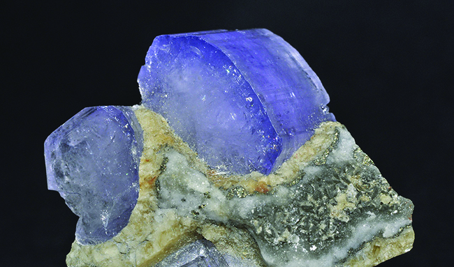
The dramatic increase in solubility with increasing acidity described above for calcium carbonate is typical of salts containing basic anions (e.g., carbonate, fluoride, hydroxide, sulfide). Another familiar example is the formation of dental cavities in tooth enamel. The major mineral component of enamel is calcium hydroxyapatite (Figure 7.4.2), a sparingly soluble ionic compound whose dissolution equilibrium is:

${\text{Ca}}_{\text{5}}\left({\text{P}{\text{O}}_{4}\right)}_{3}\text{OH}\left(s\right)\phantom{\rule{0.2em}{0ex}}$\rightleftharpoons$\phantom{\rule{0.2em}{0ex}}5{\text{Ca}}^{\text{2+}}\left(aq\right)+3{\text{PO}}_{4}{}^{\text{3−}}\left(aq\right)+{\text{OH}^-}^{\text{}}\left(aq\right)$

This figure includes an image of two large light blue apatite crystals in a mineral conglomerate that includes white, grey, and tan crystals. The blue apatite crystals have a dull, dusty, or powdered appearance. — Figure 7.4.2 – Crystal of the mineral hydroxyapatite, Ca₅(PO₄)₃OH, is shown here. The pure compound is white, but like many other minerals, this sample is colored because of the presence of impurities.

This compound dissolved to yield two different basic ions: triprotic phosphate ions:

${\text{PO}}_{4}{^{3-}}^{\text{}}\left(\mathrm{aq}\right)+{\text{H}}_{3}{\text{O}}^{+}\left(\mathrm{aq}\right)\phantom{\rule{0.2em}{0ex}}$\rightarrow$\phantom{\rule{0.2em}{0ex}}{\text{H}}_{2}{\text{PO}}_{4}{^{2-}}^{\text{}}\left(\mathrm{aq}\right)+{\text{H}}_{2}\text{O}\left(l\right)$

${\text{H}}_{2}{\text{PO}}_{4}{^{2-}}^{\text{}}\left(aq\right)+{\text{H}}_{3}{\text{O}}^{+}\left(\mathrm{aq}\right)\phantom{\rule{0.2em}{0ex}}$\rightarrow$\phantom{\rule{0.2em}{0ex}}{\text{H}}_{2}{\text{PO}}_{4}{^-}^{\text{}}\left(\mathrm{aq}\right)+{\text{H}}_{2}\text{O}\left(l\right)$

${\text{H}}_{2}{\text{PO}}_{4}{^-}^{\text{}}\left(\mathrm{aq}\right)+{\text{H}}_{3}{\text{O}}^{+}\left(\mathrm{aq}\right)\phantom{\rule{0.2em}{0ex}}$\rightarrow$\phantom{\rule{0.2em}{0ex}}{\text{H}}_{3}{\text{PO}}_{4}\left(\mathrm{aq}\right)+{\text{H}}_{2}\text{O}\left(l\right)$

and monoprotic hydroxide ions:

${\text{OH}^-}^{\text{}}\left(aq\right)+{\text{H}}_{3}{\text{O}}^{+}\phantom{\rule{0.2em}{0ex}}$\rightarrow$\phantom{\rule{0.2em}{0ex}}2{\text{H}}_{2}\text{O}$

Of the two basic productions, the hydroxide is, of course, by far the stronger base (it’s the strongest base that can exist in aqueous solution), and so it is the dominant factor providing the compound an acid-dependent solubility. Dental cavities form when the acid waste of bacteria growing on the surface of teeth hastens the dissolution of tooth enamel by reacting completely with the strong base hydroxide, shifting the hydroxyapatite solubility equilibrium to the right. Some toothpastes and mouth rinses contain added NaF or SnF₂ that make enamel more acid resistant by replacing the strong base hydroxide with the weak base fluoride:

$\text{NaF}+{\text{Ca}}_{\text{5}}\left({\text{P}{\text{O}}_{4}\right)}_{3}\text{OH}\phantom{\rule{0.2em}{0ex}}$\rightleftharpoons$\phantom{\rule{0.2em}{0ex}}{\text{Ca}}_{\text{5}}\left({\text{P}{\text{O}}_{4}\right)}_{3}\text{F}+{\text{Na}}^{+}+{\text{OH}^-}^{\text{}}$

The weak base fluoride ion reacts only partially with the bacterial acid waste, resulting in a less extensive shift in the solubility equilibrium and an increased resistance to acid dissolution. See the Chemistry in Everyday Life feature on the role of fluoride in preventing tooth decay for more information.

Role of Fluoride in Preventing Tooth Decay

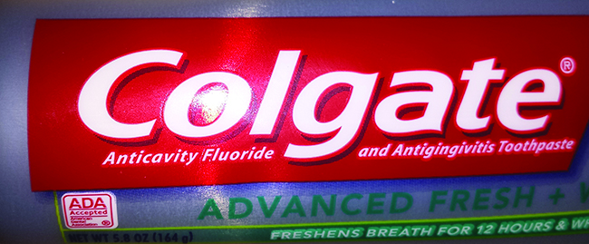
As we saw previously, fluoride ions help protect our teeth by reacting with hydroxylapatite to form fluorapatite, Ca₅(PO₄)₃F. Since it lacks a hydroxide ion, fluorapatite is more resistant to attacks by acids in our mouths and is thus less soluble, protecting our teeth. Scientists discovered that naturally fluorinated water could be beneficial to your teeth, and so it became common practice to add fluoride to drinking water. Toothpastes and mouthwashes also contain amounts of fluoride (Figure 7.4.3).

Replace with updated art; figure in “99” art folder is current and correct — **Figure 7.4.3 – Fluoride, found in many toothpastes, helps prevent tooth decay (credit: Kerry Ceszyk).**

Unfortunately, excess fluoride can negate its advantages. Natural sources of drinking water in various parts of the world have varying concentrations of fluoride, and places where that concentration is high are prone to certain health risks when there is no other source of drinking water. The most serious side effect of excess fluoride is the bone disease, skeletal fluorosis. When excess fluoride is in the body, it can cause the joints to stiffen and the bones to thicken. It can severely impact mobility and can negatively affect the thyroid gland. Skeletal fluorosis is a condition that over 2.7 million people suffer from across the world. So while fluoride can protect our teeth from decay, the US Environmental Protection Agency sets a maximum level of 4 ppm (4 mg/L) of fluoride in drinking water in the US. Fluoride levels in water are not regulated in all countries, so fluorosis is a problem in areas with high levels of fluoride in the groundwater.

The solubility of ionic compounds may also be increased when dissolution is coupled to the formation of a complex ion. For example, aluminum hydroxide dissolves in a solution of sodium hydroxide or another strong base because of the formation of the complex ion $\text{Al}{\left(\text{OH}\right)}_{4}{^-}^{\text{}}.$

An H atom is bonded to an O atom. The O atom has 2 dots above it and 2 dots below it. The O atom is bonded to an A l atom, which has three additional O atoms bonded to it as well. Each of these additional O atoms has 4 dots arranged around it, and is bonded to an H atom. This entire molecule is contained in brackets, to the right of which is a superscripted negative sign. 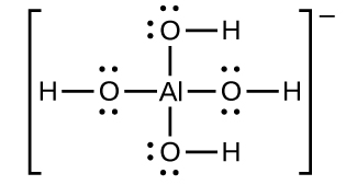— **Scheme 7.4.1 – Structure of the complex ion that forms when sodium hydroxide dissolves in a solution of sodium hydroxide.**

The equations for the dissolution of aluminum hydroxide, the formation of the complex ion, and the combined (net) equation are shown below. As indicated by the relatively large value of K for the net reaction, coupling complex formation with dissolution drastically increases the solubility of Al(OH)₃.

$\begin{array}{ccc}\hfill \text{Al}{\left(\text{OH}\right)}_{3}\left(s\right)\phantom{\rule{0.2em}{0ex}}{\rightleftharpoons}\phantom{\rule{0.2em}{0ex}}{\text{Al}}^{\text{3+}}\left(aq\right)+3{\text{OH}^-}^{\text{}}\left(aq\right)\hfill & & \hfill {K}_{\text{sp}}=2\phantom{\rule{0.2em}{0ex}}\times\phantom{\rule{0.2em}{0ex}}{10}^{-32}\hfill \\ \hfill {\text{Al}}^{\text{3+}}\left(aq\right)+4{\text{OH}^-}^{\text{}}\left(aq\right)\phantom{\rule{0.2em}{0ex}}{\rightleftharpoons}\phantom{\rule{0.2em}{0ex}}\text{Al}{\left(\text{OH}\right)}_{4}{^-}^{\text{}}\left(aq\right)\hfill & & \hfill {K}_{\text{f}}=1.1\phantom{\rule{0.2em}{0ex}}\times\phantom{\rule{0.2em}{0ex}}{10}^{33}\hfill \\ \hfill \text{Net:}\phantom{\rule{0.2em}{0ex}}\text{Al}{\left(\text{OH}\right)}_{3}\left(s\right)+{\text{OH}^-}^{\text{}}\left(aq\right)\phantom{\rule{0.2em}{0ex}}{\rightleftharpoons}\phantom{\rule{0.2em}{0ex}}\text{Al}{\left(\text{OH}\right)}_{4}{^-}^{\text{}}\left(aq\right)\hfill & & \hfill K={K}_{\text{sp}}\phantom{\rule{0.2em}{0ex}}{K}_{\text{f}}=22\hfill \end{array}$

Activity 7.4.1 – Increased Solubility in Acidic Solutions

Compute and compare the molar solublities for aluminum hydroxide, Ca(OH)₂, dissolved in (a) pure water and (b) a buffer containing 0.100 M acetic acid and 0.100 M sodium acetate.

Solution

(a) The molar solubility of calcium fluoride in water is computed considering the dissolution equilibrium only as demonstrated in several previous examples:

$\begin{array}{l}\hfill \text{Al}{\left(\text{OH}\right)}_{3}\left(s\right)\phantom{\rule{0.2em}{0ex}}{\rightleftharpoons}\phantom{\rule{0.2em}{0ex}}{\text{Al}}^{\text{3+}}\left(aq\right)+3{\text{OH}^-}^{\text{}}\left(aq\right)\hfill & & \hfill {K}_{\text{sp}}=2\phantom{\rule{0.2em}{0ex}}\times\phantom{\rule{0.2em}{0ex}}{10}^{-32}\hfill \\ \text{molar solubility in water}\phantom{\rule{0.2em}{0ex}}=\phantom{\rule{0.2em}{0ex}}\left[{\text{Al}}^{3+}\right]\phantom{\rule{0.2em}{0ex}}=\phantom{\rule{0.2em}{0ex}}{\left(2\phantom{\rule{0.2em}{0ex}}\times\phantom{\rule{0.2em}{0ex}}{10}^{-32}\phantom{\rule{0.2em}{0ex}}\text{/}\phantom{\rule{0.2em}{0ex}}27\right)}^{1\phantom{\rule{0.2em}{0ex}}\text{/}\phantom{\rule{0.2em}{0ex}}3}\phantom{\rule{0.2em}{0ex}}=\phantom{\rule{0.2em}{0ex}}9\phantom{\rule{0.2em}{0ex}}\times\phantom{\rule{0.2em}{0ex}}{10}^{-12}\phantom{\rule{0.2em}{0ex}}M\end{array}$

(b) The concentration of hydroxide ion of the buffered solution is conveniently calculated by the Henderson-Hasselbalch equation:

$\begin{array}{l}\text{pH}\phantom{\rule{0.2em}{0ex}}=\phantom{\rule{0.2em}{0ex}}{\text{pK}}_{\text{a}}\phantom{\rule{0.2em}{0ex}}+\phantom{\rule{0.2em}{0ex}}\text{log}\phantom{\rule{0.2em}{0ex}}\left[{\text{CH}}_{3}{\text{COO}}^{-}\right]\phantom{\rule{0.2em}{0ex}}\text{/}\phantom{\rule{0.2em}{0ex}}\left[{\text{CH}}_{3}\text{COOH}\right]\\ \\ \text{pH}\phantom{\rule{0.2em}{0ex}}=\phantom{\rule{0.2em}{0ex}}4.74\phantom{\rule{0.2em}{0ex}}+\phantom{\rule{0.2em}{0ex}}\text{log}\phantom{\rule{0.2em}{0ex}}\left(0.100\phantom{\rule{0.2em}{0ex}}\text{/}\phantom{\rule{0.2em}{0ex}}0.100\right)\phantom{\rule{0.2em}{0ex}}=\phantom{\rule{0.2em}{0ex}}4.74\end{array}$

At this pH, the concentration of hydroxide ion is:

$\begin{array}{l}\text{pOH}\phantom{\rule{0.2em}{0ex}}=\phantom{\rule{0.2em}{0ex}}14.00\phantom{\rule{0.2em}{0ex}}-\phantom{\rule{0.2em}{0ex}}4.74\phantom{\rule{0.2em}{0ex}}=\phantom{\rule{0.2em}{0ex}}9.26\\ \left[{\text{OH}}^{-}\right]\phantom{\rule{0.2em}{0ex}}=\phantom{\rule{0.2em}{0ex}}{10}^{-9.26}\phantom{\rule{0.2em}{0ex}}=\phantom{\rule{0.2em}{0ex}}5.5\phantom{\rule{0.2em}{0ex}}\times\phantom{\rule{0.2em}{0ex}}{10}^{-10}\end{array}$

The solubility of Al(OH)₃ in this buffer is then calculated from its solubility product expressions:

$\begin{array}{l}\hfill {K}_{\text{sp}}\phantom{\rule{0.2em}{0ex}}=\phantom{\rule{0.2em}{0ex}}\left[{\text{Al}}^{3+}\right]{\left[{\text{OH}}^{-}\right]}^{3}\hfill \\ \text{molar solubility in buffer}\phantom{\rule{0.2em}{0ex}}=\phantom{\rule{0.2em}{0ex}}\left[{\text{Al}}^{3+}\right]\phantom{\rule{0.2em}{0ex}}=\phantom{\rule{0.2em}{0ex}}{K}_{\text{sp}}\phantom{\rule{0.2em}{0ex}}\text{/}\phantom{\rule{0.2em}{0ex}}{\left[{\text{OH}}^{-}\right]}^{3}\phantom{\rule{0.2em}{0ex}}=\phantom{\rule{0.2em}{0ex}}\left(2\phantom{\rule{0.2em}{0ex}}\times\phantom{\rule{0.2em}{0ex}}{10}^{-32}\right)\phantom{\rule{0.2em}{0ex}}\text{/}\phantom{\rule{0.2em}{0ex}}{\left(5.5\phantom{\rule{0.2em}{0ex}}\times\phantom{\rule{0.2em}{0ex}}{10}^{-10}\right)}^{3}\phantom{\rule{0.2em}{0ex}}=\phantom{\rule{0.2em}{0ex}}1.2\phantom{\rule{0.2em}{0ex}}\times\phantom{\rule{0.2em}{0ex}}{10}^{-4}\phantom{\rule{0.2em}{0ex}}M\end{array}$

Compared to pure water, the solubility of aluminum hydroxide in this mildly acidic buffer is approximately ten million times greater (though still relatively low).

Check Your Learning

What is the solubility of aluminum hydroxide in a buffer comprised of 0.100 M formic acid and 0.100 M sodium formate?

Answer

0.1 M

Activity 7.4.2 – Multiple Equilibria

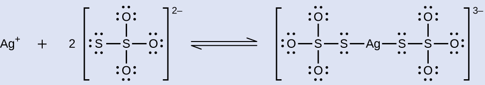
Unexposed silver halides are removed from photographic film when they react with sodium thiosulfate (Na₂S₂O₃, called hypo) to form the complex ion $\left[\text{Ag}{\left({\text{S}}_{2}{\text{O}}_{3}\right)}_{2}\right]{^{3-}}^{\text{}}$ (K_f = 4.7 $\times\times$ 10¹³).

What mass of Na₂S₂O₃ is required to prepare 1.00 L of a solution that will dissolve 1.00 g of AgBr by the formation of $\left[\text{Ag}{\left({\text{S}}_{2}{\text{O}}_{3}\right)}_{2}\right]{^{3-}}^{\text{}}$

Solution

Two equilibria are involved when AgBr dissolves in a solution containing the ${\text{S}}_{2}{\text{O}}_{3}{^{2-}}^{\text{}}$ ion:

dissolution: $\text{AgBr}\left(s\right)$\rightleftharpoons${\text{Ag}}^{\text{+}}\left(aq\right)+{\text{Br}^-}^{\text{}}\left(aq\right)\phantom{\rule{4em}{0ex}}{K}_{\text{sp}}=5.0\phantom{\rule{0.2em}{0ex}}\times\phantom{\rule{0.2em}{0ex}}{10}^{-13}$

complexation: ${\text{Ag}}^{\text{+}}\left(aq\right)+{\text{2S}}_{2}{\text{O}}_{3}{^{2-}}^{\text{}}\left(aq\right)$\rightleftharpoons$\left[\text{Ag}{\left({\text{S}}_{2}{\text{O}}_{3}\right)}_{2}\right]{^{3-}}^{\text{}}\left(aq\right)\phantom{\rule{4em}{0ex}}{K}_{\text{f}}=4.7\phantom{\rule{0.2em}{0ex}}\times\phantom{\rule{0.2em}{0ex}}{10}^{13}$

First, calculate the concentration of bromide that will result when the 1.00 g of AgBr is completely dissolved via the cited complexation reaction:

$\begin{array}{l}1.00\phantom{\rule{0.2em}{0ex}}\text{g}\phantom{\rule{0.2em}{0ex}}\text{AgBr}\phantom{\rule{0.2em}{0ex}}\text{/}\phantom{\rule{0.2em}{0ex}}\left(187.77\phantom{\rule{0.2em}{0ex}}\text{g}\text{/}\text{mol}\right)\left(1\phantom{\rule{0.2em}{0ex}}\text{mol}\phantom{\rule{0.2em}{0ex}}{\text{Br}^-}^{}\phantom{\rule{0.2em}{0ex}}\text{/}\phantom{\rule{0.2em}{0ex}}1\phantom{\rule{0.2em}{0ex}}\text{mol}\phantom{\rule{0.2em}{0ex}}\text{AgBr}\right)\phantom{\rule{0.2em}{0ex}}=\phantom{\rule{0.2em}{0ex}}0.00532\phantom{\rule{0.2em}{0ex}}\text{mol}\phantom{\rule{0.2em}{0ex}}{\text{Br}^-}^{}\\ 0.00521\phantom{\rule{0.2em}{0ex}}\text{mol}\phantom{\rule{0.2em}{0ex}}{\text{Br}^-}^{}\phantom{\rule{0.2em}{0ex}}\text{/}\phantom{\rule{0.2em}{0ex}}1.00\phantom{\rule{0.2em}{0ex}}\text{L}\phantom{\rule{0.2em}{0ex}}=\phantom{\rule{0.2em}{0ex}}0.00521\phantom{\rule{0.2em}{0ex}}M\phantom{\rule{0.2em}{0ex}}{\text{Br}^-}^{}\end{array}$

Next, use this bromide molarity and the solubility product for silver bromide to calculate the silver ion molarity in the solution:

$\left[{\text{Ag}}^{+}\right]\phantom{\rule{0.2em}{0ex}}=\phantom{\rule{0.2em}{0ex}}{K}_{\text{sp}}\phantom{\rule{0.2em}{0ex}}\text{/}\phantom{\rule{0.2em}{0ex}}\left[{\text{Br}^-}^{}\right]\phantom{\rule{0.2em}{0ex}}=\phantom{\rule{0.2em}{0ex}}5.0\phantom{\rule{0.2em}{0ex}}\times\phantom{\rule{0.2em}{0ex}}{10}^{-13}\phantom{\rule{0.2em}{0ex}}\text{/}\phantom{\rule{0.2em}{0ex}}0.00521\phantom{\rule{0.2em}{0ex}}=\phantom{\rule{0.2em}{0ex}}9.6\phantom{\rule{0.2em}{0ex}}\times\phantom{\rule{0.2em}{0ex}}{10}^{-11}\phantom{\rule{0.2em}{0ex}}M$

Based on the stoichiometry of the complex ion formation, the concentration of complex ion produced is:

$0.00521\phantom{\rule{0.2em}{0ex}}-\phantom{\rule{0.2em}{0ex}}9.6\phantom{\rule{0.2em}{0ex}}\times\phantom{\rule{0.2em}{0ex}}{10}^{-11}\phantom{\rule{0.2em}{0ex}}=\phantom{\rule{0.2em}{0ex}}0.00521\phantom{\rule{0.2em}{0ex}}M$

Use the silver ion and complex ion concentrations and the formation constant for the complex ion to compute the concentration of thiosulfate ion:

$\begin{array}{l}{\left[{{\text{S}}_{2}{\text{O}}_{3}{^{2-}}\right]}^{2}\phantom{\rule{0.2em}{0ex}}=\phantom{\rule{0.2em}{0ex}}\left[\text{Ag}{\left({\text{S}}_{2}{\text{O}}_{3}\right)}_{2}\right]}^{3-}\right]\text{/}\left[{\text{Ag}}^{+}\right]{K}_{\text{f}}\phantom{\rule{0.2em}{0ex}}=\phantom{\rule{0.2em}{0ex}}0.00521\text{/}\left(9.6\phantom{\rule{0.2em}{0ex}}\times\phantom{\rule{0.2em}{0ex}}{10}^{-11}\right)\left(4.7\phantom{\rule{0.2em}{0ex}}\times\phantom{\rule{0.2em}{0ex}}{10}^{13}\right)\phantom{\rule{0.2em}{0ex}}=\phantom{\rule{0.2em}{0ex}}1.15\phantom{\rule{0.2em}{0ex}}\times\phantom{\rule{0.2em}{0ex}}{10}^{-6}\\ \left[{{\text{S}}_{2}{\text{O}}_{3}{^{2-}}^{}\right]\phantom{\rule{0.2em}{0ex}}=\phantom{\rule{0.2em}{0ex}}1.1\phantom{\rule{0.2em}{0ex}}\times\phantom{\rule{0.2em}{0ex}}{10}^{-3}\phantom{\rule{0.2em}{0ex}}M\end{array}$

Finally, use this molar concentration to derive the required mass of sodium thiosulfate:

$\left(1.1\phantom{\rule{0.2em}{0ex}}\times\phantom{\rule{0.2em}{0ex}}{10}^{-3}\phantom{\rule{0.2em}{0ex}}\text{mol}\phantom{\rule{0.2em}{0ex}}{{\text{S}}_{2}{\text{O}}_{3}^{^{2-}}^{}\phantom{\rule{0.2em}{0ex}}\text{/}\phantom{\rule{0.2em}{0ex}}\text{L}\right)\left(1\phantom{\rule{0.2em}{0ex}}\text{mol}\phantom{\rule{0.2em}{0ex}}{\text{NaS}}_{2}{\text{O}}_{3}\phantom{\rule{0.2em}{0ex}}\text{/}\phantom{\rule{0.2em}{0ex}}1\phantom{\rule{0.2em}{0ex}}\text{mol}\phantom{\rule{0.2em}{0ex}}{{\text{S}}_{2}{\text{O}}_{3}{^{2-}}^{}\right)\left(158.1\phantom{\rule{0.2em}{0ex}}\text{g}\phantom{\rule{0.2em}{0ex}}{\text{NaS}}_{2}{\text{O}}_{3}\phantom{\rule{0.2em}{0ex}}\text{/}\phantom{\rule{0.2em}{0ex}}\text{mol}\right)\phantom{\rule{0.2em}{0ex}}=\phantom{\rule{0.2em}{0ex}}1.7\phantom{\rule{0.2em}{0ex}}\text{g}$

Thus, 1.00 L of a solution prepared from 1.7 g Na₂S₂O₃ dissolves 1.0 g of AgBr.

Check Your Learning

AgCl(s), silver chloride, has a very low solubility:

$\text{AgCl}\left(s\right)$\rightleftharpoons${\text{Ag}}^{\text{+}}\left(aq\right)+{\text{Cl}^-}^{\text{}}\left(aq\right),$ K_sp = 1.6 $\times$ 10^–10.

Adding ammonia significantly increases the solubility of AgCl because a complex ion is formed:

${\text{Ag}}^{\text{+}}\left(aq\right)+2{\text{NH}}_{3}\left(aq\right)$\rightleftharpoons$\left[\text{Ag}{\left({\text{NH}}_{3}\right)}_{2}\right]{}^{+}\left(aq\right),$ K_f = 1.7 $\times$ 10⁷.

What mass of NH₃ is required to prepare 1.00 L of solution that will dissolve 2.00 g of AgCl by formation of $\text{Ag}{\left({\text{NH}}_{3}\right)}_{2}{}^{\text{+}}?$

Answer

1.00 L of a solution prepared with 4.81 g NH₃ dissolves 2.0 g of AgCl.

Systems involving two or more chemical equilibria that share one or more reactant or product are called coupled equilibria. Common examples of coupled equilibria include the increased solubility of some compounds in acidic solutions (coupled dissolution and neutralization equilibria) and in solutions containing ligands (coupled dissolution and complex formation). The equilibrium tools from other chapters may be applied to describe and perform calculations on these systems.

End of Chapter Exercises

(1) A saturated solution of a slightly soluble electrolyte in contact with some of the solid electrolyte is said to be a system in equilibrium. Explain. Why is such a system called a heterogeneous equilibrium?

(2) Calculate the equilibrium concentration of Ni²⁺ in a 1.0 M solution [Ni(NH₃)₆](NO₃)₂.

Solution

0.014 M

(3) Calculate the equilibrium concentration of Zn²⁺ in a 0.30-M solution of $\text{Zn}{\left(\text{CN}\right)}_{4}{^{2-}}^{\text{}}.$

(4) Calculate the equilibrium concentration of Cu²⁺ in a solution initially with 0.050 M Cu²⁺ and 1.00 M NH₃.

Solution

7.2 $\times$ 10^–15M

(5) Calculate the equilibrium concentration of Zn²⁺ in a solution initially with 0.150 M Zn²⁺ and 2.50 M CN^–.

(6) Calculate the Fe³⁺ equilibrium concentration when 0.0888 mole of K₃[Fe(CN)₆] is added to a solution with 0.0.00010 M CN^–.

Solution

4.4 $\times$ 10⁻²²M

(7) Calculate the Co²⁺ equilibrium concentration when 0.100 mole of [Co(NH₃)₆](NO₃)₂ is added to a solution with 0.025 M NH₃. Assume the volume is 1.00 L.

(8) Calculate the molar solubility of Sn(OH)₂ in a buffer solution containing equal concentrations of NH₃ and ${\text{NH}}_{4}{}^{+}.$

(9) Calculate the molar solubility of Al(OH)₃ in a buffer solution with 0.100 M NH₃ and 0.400 M ${\text{NH}}_{4}{}^{+}.$

Solution

[OH⁻] = 4.5 $\times$ 10⁻⁵; [Al³⁺] = 2.2 $\times$ 10^–20 (molar solubility)

(10) What is the molar solubility of CaF₂ in a 0.100-M solution of HF? K_a for HF = 6.4 $\times$ 10^–4.

(11) What is the molar solubility of BaSO₄ in a 0.250-M solution of NaHSO₄? K_a for ${\text{HSO}}_{4}{^-}^{\text{}}$ = 1.2 $\times$ 10^–2.

Solution

$\left[{\text{SO}}_{4}{^{2-}}^{\text{}}\right]=0.049\phantom{\rule{0.2em}{0ex}}M$ ; [Ba²⁺] = 4.7 $\times$ 10^–7 (molar solubility)

(12) What is the molar solubility of Tl(OH)₃ in a 0.10-M solution of NH₃?

(13) What is the molar solubility of Pb(OH)₂ in a 0.138-M solution of CH₃NH₂?

Solution

[OH^–] = 7.6 $\times$ 10⁻³M; [Pb²⁺] = 2.1 $\times$ 10^–11 (molar solubility)

(14) A solution of 0.075 M CoBr₂ is saturated with H₂S ([H₂S] = 0.10 M). What is the minimum pH at which CoS begins to precipitate?

$\text{CoS}\left(s\right)$\rightleftharpoons${\text{Co}}^{\text{2+}}\left(aq\right)+{\text{S}^{2-}}^{\text{}}\left(aq\right)\phantom{\rule{4em}{0ex}}{K}_{\text{sp}}=4.5\phantom{\rule{0.2em}{0ex}}\times\phantom{\rule{0.2em}{0ex}}{10}^{-27}$

${\text{H}}_{2}\text{S}\left(aq\right)+2{\text{H}}_{2}\text{O}\left(l\right)$\rightleftharpoons$2{\text{H}}_{3}{\text{O}}^{\text{+}}\left(aq\right)+{\text{S}^{2-}}^{\text{}}\left(aq\right)\phantom{\rule{4em}{0ex}}K=1.0\phantom{\rule{0.2em}{0ex}}\times\phantom{\rule{0.2em}{0ex}}{10}^{-26}$

(15) A 0.125-M solution of Mn(NO₃)₂ is saturated with H₂S ([H₂S] = 0.10 M). At what pH does MnS begin to precipitate?

$\text{MnS}\left(s\right)$\rightleftharpoons${\text{Mn}}^{\text{2+}}\left(aq\right)+{\text{S}^{2-}}^{\text{}}\left(aq\right)\phantom{\rule{4em}{0ex}}{K}_{\text{sp}}=4.3\phantom{\rule{0.2em}{0ex}}\times\phantom{\rule{0.2em}{0ex}}{10}^{-22}$

${\text{H}}_{2}\text{S}\left(aq\right)+2{\text{H}}_{2}\text{O}\left(l\right)$\rightleftharpoons$2{\text{H}}_{3}{\text{O}}^{\text{+}}\left(aq\right)+{\text{S}^{2-}}^{\text{}}\left(aq\right)\phantom{\rule{4em}{0ex}}K=1.0\phantom{\rule{0.2em}{0ex}}\times\phantom{\rule{0.2em}{0ex}}{10}^{-26}$

Solution

7.66

(16) Both AgCl and AgI dissolve in NH₃.

(16a) What mass of AgI dissolves in 1.0 L of 1.0 M NH₃?

(16b) What mass of AgCl dissolves in 1.0 L of 1.0 M NH₃?

The following question is taken from a Chemistry Advanced Placement Examination and is used with the permission of the Educational Testing Service.

(17) Solve the following problem:

${\text{MgF}}_{2}\left(s\right)$\rightleftharpoons${\text{Mg}}^{\text{2+}}\left(aq\right)+2{\text{F}^-}^{\text{}}\left(aq\right)$

In a saturated solution of MgF₂ at 18 °C, the concentration of Mg²⁺ is 1.21 $\times$ 10^–3M. The equilibrium is represented by the preceding equation.

(17a) Write the expression for the solubility-product constant, K_sp, and calculate its value at 18 °C.

(17b) Calculate the equilibrium concentration of Mg²⁺ in 1.000 L of saturated MgF₂ solution at 18 °C to which 0.100 mol of solid KF has been added. The KF dissolves completely. Assume the volume change is negligible.

(17c) Predict whether a precipitate of MgF₂ will form when 100.0 mL of a 3.00 $\times$ 10^–3–M solution of Mg(NO₃)₂ is mixed with 200.0 mL of a 2.00 $\times$ 10^–3–M solution of NaF at 18 °C. Show the calculations to support your prediction.

(17d) At 27 °C the concentration of Mg²⁺ in a saturated solution of MgF₂ is 1.17 $\times$ 10^–3M. Is the dissolving of MgF₂ in water an endothermic or an exothermic process? Give an explanation to support your conclusion.

Solution

(a) K_sp = [Mg²⁺][F^–]² = (1.21 $\times$ 10^–3)(2 $\times$ 1.21 $\times$ 10^–3)² = 7.09 $\times$ 10^–9

(b) 7.09 $\times$ 10^–7M

(c) Determine the concentration of Mg²⁺ and F^– that will be present in the final volume. Compare the value of the ion product [Mg²⁺][F^–]² with K_sp. If this value is larger than K_sp, precipitation will occur.

0.1000 L $\times$ 3.00 $\times$ 10^–3M Mg(NO₃)₂ = 0.3000 L $\times$ M Mg(NO₃)₂

M Mg(NO₃)₂ = 1.00 $\times$ 10^–3M

0.2000 L $\times$ 2.00 $\times$ 10^–3M NaF = 0.3000 L $\times$ M NaF

M NaF = 1.33 $\times$ 10^–3M

ion product = (1.00 $\times$ 10^–3)(1.33 $\times$ 10^–3)² = 1.77 $\times$ 10^–9 This value is smaller than K_sp, so no precipitation will occur.

(d) MgF₂ is less soluble at 27 °C than at 18 °C. Because added heat acts like an added reagent, when it appears on the product side, the Le Châtelier’s principle states that the equilibrium will shift to the reactants’ side to counter the stress. Consequently, less reagent will dissolve. This situation is found in our case. Therefore, the reaction is exothermic.

(18) Which of the following compounds, when dissolved in a 0.01-M solution of HClO₄, has a solubility greater than in pure water: CuCl, CaCO₃, MnS, PbBr₂, CaF₂? Explain your answer.

(19) Which of the following compounds, when dissolved in a 0.01-M solution of HClO₄, has a solubility greater than in pure water: AgBr, BaF₂, Ca₃(PO₄)₂, ZnS, PbI₂? Explain your answer.

Solution

BaF₂, Ca₃(PO₄)₂, ZnS; each is a salt of a weak acid, and the $\left[{\text{H}}_{3}{\text{O}}^{+}\right]$ from perchloric acid reduces the equilibrium concentration of the anion, thereby increasing the concentration of the cations.

(20) What is the effect on the amount of solid Mg(OH)₂ that dissolves and the concentrations of Mg²⁺ and OH^– when each of the following are added to a mixture of solid Mg(OH)₂ and water at equilibrium?

(20a) MgCl₂

(20b) KOH

(20c) HClO₄

(20d) NaNO₃

(20e) Mg(OH)₂

(21) What is the effect on the amount of CaHPO₄ that dissolves and the concentrations of Ca²⁺ and ${\text{HPO}}_{4}{^-}^{\text{}}$ when each of the following are added to a mixture of solid CaHPO₄ and water at equilibrium?

(21a) CaCl₂

(21b) HCl

(21c) KClO₄

(21d) NaOH

(21e) CaHPO₄

Solution

Effect on amount of solid CaHPO₄, [Ca²⁺], [OH^–]: (a) increase, increase, decrease; (b) decrease, increase, decrease; (c) no effect, no effect, no effect; (d) decrease, increase, decrease; (e) increase, no effect, no effect

(22) Identify all chemical species present in an aqueous solution of Ca₃(PO₄)₂ and list these species in decreasing order of their concentrations. (Hint: Remember that the ${\text{PO}}_{4}{^{3-}}^{\text{}}$ ion is a weak base.)

Glossary

coupled equilibria: system characterized the simultaneous establishment of two or more equilibrium reactions sharing one or more reactant or product

License

Icon for the Creative Commons Attribution 4.0 International License

Inorganic Chemistry for Chemical Engineers Copyright © 2020 by Vishakha Monga; Paul Flowers; Klaus Theopold; William R. Robinson; and Richard Langley is licensed under a Creative Commons Attribution 4.0 International License, except where otherwise noted.

Role of Fluoride in Preventing Tooth Decay

Solution

Check Your Learning

Answer

Solution

Check Your Learning

Answer

Key Concepts and Summary

Glossary

License

Share This Book