10.6 Graphing Quadratic Equations—Vertex and Intercept Method

Terrance Berg

Chapter 10: Quadratics

10.6 Graphing Quadratic Equations—Vertex and Intercept Method

One useful strategy that is used to get a quick sketch of a quadratic equation is to identify 3 key points of the quadratic: its vertex and the two intercept points. From these 3 points, it’s possible to sketch out a rough graph of what the quadratic graph looks like.

The intercepts are where the quadratic equation crosses the $x$ -axis and are found when the quadratic is set to equal 0. So instead of the quadratic looking like $y = ax^2 + bx + c$ , it is instead factored from the form $0 = ax^2 + bx + c$ to get its $x$ -intercepts (roots). For expedience, you can get these values using the quadratic equation.

$x=\dfrac{-b\pm (b^2-4ac)^{\frac{1}{2}}}{2a}$

The vertex is found by using the quadratic equation where the discriminant equals zero, which gives us the $x$ -coordinate of $x = \dfrac{-b}{2a}$ . The $y$ -coordinate of the vertex is then found by placing the $x$ -coordinate of the vertex $\left(x = \dfrac{-b}{2a}\right)$ back into the original quadratic $(y = ax^2 + bx + c)$ and solving for $y$ .

The vertex then takes the form of $\left[\dfrac{-b}{2a}, a\left(\dfrac{-b}{2a}\right)^2 + \left(\dfrac{-b}{2a}\right)x + c\right]$ , or simply as $\left[\dfrac{-b}{2a}, f\left(\dfrac{-b}{2a}\right)\right].$

What is new here is finding the vertex, so consider the following examples.

Example 10.6.1

Find the vertex of $y = x^2 + 6x - 7$ .

For this equation, $a = 1$ , $b = 6$ and $c = -7$ .

This means that the $x$ -coordinate of the vertex $x = \dfrac{-b}{2a}$ will give us the value $x = \dfrac{-(6)}{2(1)}= -3$ .

We now use this $x$ -coordinate to find the $y$ -coordinate.

$\begin{array}{ccccccc} y&=&ax^2&+&bx&+&c \\ y&=&1(-3)^2&+&6(-3)&-&7 \\ y&=&9&-&18&-&7 \\ y&=&-16&&&& \end{array}$

The vertex is at $x = -3$ and $y = -16$ and can be given by the coordinate $(-3, -16)$ .

The $x$ -intercepts or roots of the quadratic in Example 10.6.1 are found by factoring $x^2 + 6x - 7 = 0$ .

For this problem, the quadratic factors to $(x + 7)(x - 1) = 0$ , which means the roots are $x = -7$ and $x = 1$ . Putting all this data together gives us the vertex coordinate $(-3, -16)$ and the two $x$ -intercept coordinates $(-7, 0)$ and $(1, 0)$ . These are the values used to create the rough sketch.

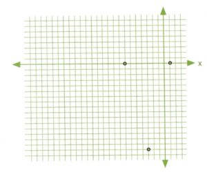two x-intercept coordinates (-7, 0) and (1, 0) Trying to sketch this curve will be somewhat challenging if there is to be any semblance of accuracy.

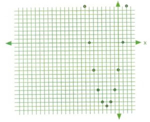
When this happens, it is quite easy to fill in some of the places where there may have been coordinates by using a data table.

For this graph, choose values from $x = 2$ to $x = -8$ .

First, find the value of $y$ when $x=2$ :

$\begin{array}{rrrrrrr} y&=&x^2&+&6x&-&7 \\ y&=&1(2)^2&+&6(2)&-&7 \\ y&=&4&+&12&-&7 \\ y&=&9&&&& \end{array}$

Put this value in the table and then carry on to complete all of it.

$x$	$y$
2	9
1	0
0	−7
−1	−12
−2	−15
−3	−16
−4	−15
−5	−12
−6	−7
−7	0
−8	9

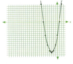
Placing all of these coordinates on the graph will generate a graph showing increased detail, as shown below. All that remains is to draw a curve that connects the points on the graph. The level of detail required to draw the curve only depends on the unique characteristics of the curve itself.

Remember:

For the quadratic equation $y = ax^2 + bx + c$ , the $x$ -coordinate of the vertex is $x = \dfrac{-b}{2a}$ and the $y$ -coordinate of the vertex is $y = a \left(\dfrac{-b}{2a}\right)^2 + \left(\dfrac{-b}{2a}\right)x + c$ .

The following questions will ask you to sketch the quadratic function using the vertex and the x-intercepts and then later to draw a data table to find the coordinates of data points from which to draw a curve.

Both approaches are quite valuable, the difference is only in the details, which if required can use both techniques to general a curve in increased detail.

Example 10.6.2

Find the vertex of $y = x^2 - 6x - 7$ .

In the equation, $a = 1$ , $b = -6$ , and $c = -7$ .

This means that the $x$ -coordinate of the vertex $x = \dfrac{-b}{2a}$ will give us the value $x = \dfrac{-(-6)}{2}(1)$ or 3.

We now use this $x$ -coordinate to find the $y$ -coordinate.

$\begin{array}{rrrrrrr} y&=&ax^2&+&bx&+&c \\ y&=&1(3)^2&-&6(3)&-&7 \\ y&=&9&-&18&-&7 \\ y&=&-16&&&& \end{array}$

The vertex is at $x = +3$ and $y = -16$ and can be given by the coordinate $(+3, -16)$ .

The $x$ -intercepts or roots of this quadratic are found by factoring $x^2 + 6x - 7 = 0$ .

For this problem, the quadratic factors to $(x - 7)(x + 1) = 0$ , which means the roots are $x = +7$ and $x = -1$ . Putting all this data together gives us the vertex coordinate $(-3, -16)$ and the two $x$ -intercept coordinates $(7, 0)$ and $(-1, 0)$ .

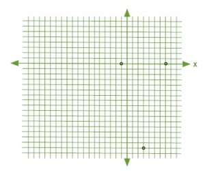Trying to sketch this curve will be somewhat challenging if there is to be any semblance of accuracy.

When this happens, it is quite easy to fill in some of the places where there may have been coordinates by using a data table.

For this graph, choose values for $x = 0$ to $x = 6$ . First, find the value of $y$ when $x = 0$ :

$\begin{array}{rrrrrrr} y&=&x^2&-&6x&-&7 \\ y&=&(0)^2&-&6(0)&-&7 \\ y&=&0&-&0&-&7 \\ y&=&-7&&&& \end{array}$

Put this value in the table and then carry on to complete all of it.

$x$	$y$
5	7
4	0
3	−5
2	−8
1	−9
0	−8
−1	−5
−2	0
−3	7

Placing all of these coordinates on the graph will generate a graph showing increased detail as shown below. All that remains is to draw a curve that connects the points on the graph. The level of detail you require to draw the curve only depends on the unique characteristics of the curve itself.

Remember:

For the quadratic equation $y = ax^2 + bx + c$ , the $x$ -coordinate of the vertex is $x = \dfrac{-b}{2a}$ and the $y$ -coordinate of the vertex is $y = a \left(\dfrac{-b}{2a}\right)^2 + \left(\dfrac{-b}{2a}\right)x + c$ .

The following questions will ask you to sketch the quadratic function using the vertex and the $x$ -intercepts, and then later to draw a data table to find the coordinates of data points with which to draw a curve.

Both approaches are quite valuable. The difference is only in the detail. If required, you can use both techniques to generate a curve in increased detail.

Questions

Find the vertex and intercepts of the following quadratics. Use this information to graph the quadratic.

$y=x^2-2x-8$
$y=x^2-2x-3$
$y=2x^2-12x+10$
$y=2x^2-12x+16$
$y=-2x^2+12x-18$
$y=-2x^2+12x-10$
$y=-3x^2+24x-45$
$y=-2(x^2+2x)+6$

First, find the line of symmetry for each of the following equations. Then, construct a data table for each equation. Use this table to graph the equation.

$y=3x^2-6x-5$
$y=2x^2-4x-3$
$y=-x^2+4x+2$
$y=-3x^2-6x+2$

Answer Key 10.6

License

Icon for the Creative Commons Attribution-NonCommercial-ShareAlike 4.0 International License

Questions

License

Share This Book