Chapter 19 Celestial Distances
19.4 The H–R Diagram and Cosmic Distances
Learning Objectives
By the end of this section, you will be able to:
- Understand how spectral types are used to estimate stellar luminosities
- Examine how these techniques are used by astronomers today
Variable stars are not the only way that we can estimate the luminosity of stars. Another way involves the H–R diagram, which shows that the intrinsic brightness of a star can be estimated if we know its spectral type.
Distances from Spectral Types
As satisfying and productive as variable stars have been for distance measurement, these stars are rare and are not found near all the objects to which we wish to measure distances. Suppose, for example, we need the distance to a star that is not varying, or to a group of stars, none of which is a variable. In this case, it turns out the H–R diagram can come to our rescue.
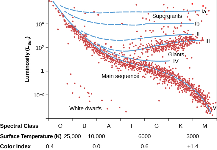
If we can observe the spectrum of a star, we can estimate its distance from our understanding of the H–R diagram. As discussed in Analyzing Starlight, a detailed examination of a stellar spectrum allows astronomers to classify the star into one of the spectral types indicating surface temperature. (The types are O, B, A, F, G, K, M, L, T, and Y; each of these can be divided into numbered subgroups.) In general, however, the spectral type alone is not enough to allow us to estimate luminosity. Look again at [link]. A G2 star could be a main-sequence star with a luminosity of 1 LSun, or it could be a giant with a luminosity of 100 LSun, or even a supergiant with a still higher luminosity.
We can learn more from a star’s spectrum, however, than just its temperature. Remember, for example, that we can detect pressure differences in stars from the details of the spectrum. This knowledge is very useful because giant stars are larger (and have lower pressures) than main-sequence stars, and supergiants are still larger than giants. If we look in detail at the spectrum of a star, we can determine whether it is a main-sequence star, a giant, or a supergiant.
Suppose, to start with the simplest example, that the spectrum, color, and other properties of a distant G2 star match those of the Sun exactly. It is then reasonable to conclude that this distant star is likely to be a main-sequence star just like the Sun and to have the same luminosity as the Sun. But if there are subtle differences between the solar spectrum and the spectrum of the distant star, then the distant star may be a giant or even a supergiant.
The most widely used system of star classification divides stars of a given spectral class into six categories called luminosity classes. These luminosity classes are denoted by Roman numbers as follows:
- Ia: Brightest supergiants
- Ib: Less luminous supergiants
- II: Bright giants
- III: Giants
- IV: Subgiants (intermediate between giants and main-sequence stars)
- V: Main-sequence stars
The full spectral specification of a star includes its luminosity class. For example, a main-sequence star with spectral class F3 is written as F3 V. The specification for an M2 giant is M2 III. [link] illustrates the approximate position of stars of various luminosity classes on the H–R diagram. The dashed portions of the lines represent regions with very few or no stars.
With both its spectral and luminosity classes known, a star’s position on the H–R diagram is uniquely determined. Since the diagram plots luminosity versus temperature, this means we can now read off the star’s luminosity (once its spectrum has helped us place it on the diagram). As before, if we know how luminous the star really is and see how dim it looks, the difference allows us to calculate its distance. (For historical reasons, astronomers sometimes call this method of distance determination spectroscopic parallax, even though the method has nothing to do with parallax.)
The H–R diagram method allows astronomers to estimate distances to nearby stars, as well as some of the most distant stars in our Galaxy, but it is anchored by measurements of parallax. The distances measured using parallax are the gold standard for distances: they rely on no assumptions, only geometry. Once astronomers take a spectrum of a nearby star for which we also know the parallax, we know the luminosity that corresponds to that spectral type. Nearby stars thus serve as benchmarks for more distant stars because we can assume that two stars with identical spectra have the same intrinsic luminosity.
A Few Words about the Real World
Introductory textbooks such as ours work hard to present the material in a straightforward and simplified way. In doing so, we sometimes do our students a disservice by making scientific techniques seem too clean and painless. In the real world, the techniques we have just described turn out to be messy and difficult, and often give astronomers headaches that last long into the day.
For example, the relationships we have described such as the period-luminosity relation for certain variable stars aren’t exactly straight lines on a graph. The points representing many stars scatter widely when plotted, and thus, the distances derived from them also have a certain built-in scatter or uncertainty.
The distances we measure with the methods we have discussed are therefore only accurate to within a certain percentage of error—sometimes 10%, sometimes 25%, sometimes as much as 50% or more. A 25% error for a star estimated to be 10,000 light-years away means it could be anywhere from 7500 to 12,500 light-years away. This would be an unacceptable uncertainty if you were loading fuel into a spaceship for a trip to the star, but it is not a bad first figure to work with if you are an astronomer stuck on planet Earth.
Nor is the construction of H–R diagrams as easy as you might think at first. To make a good diagram, one needs to measure the characteristics and distances of many stars, which can be a time-consuming task. Since our own solar neighborhood is already well mapped, the stars astronomers most want to study to advance our knowledge are likely to be far away and faint. It may take hours of observing to obtain a single spectrum. Observers may have to spend many nights at the telescope (and many days back home working with their data) before they get their distance measurement. Fortunately, this is changing because surveys like Gaia will study billions of stars, producing public datasets that all astronomers can use.
Despite these difficulties, the tools we have been discussing allow us to measure a remarkable range of distances—parallaxes for the nearest stars, RR Lyrae variable stars; the H–R diagram for clusters of stars in our own and nearby galaxies; and cepheids out to distances of 60 million light-years. [link] describes the distance limits and overlap of each method.
Each technique described in this chapter builds on at least one other method, forming what many call the cosmic distance ladder. Parallaxes are the foundation of all stellar distance estimates, spectroscopic methods use nearby stars to calibrate their H–R diagrams, and RR Lyrae and cepheid distance estimates are grounded in H–R diagram distance estimates (and even in a parallax measurement to a nearby cepheid, Delta Cephei).
This chain of methods allows astronomers to push the limits when looking for even more distant stars. Recent work, for example, has used RR Lyrae stars to identify dim companion galaxies to our own Milky Way out at distances of 300,000 light-years. The H–R diagram method was recently used to identify the two most distant stars in the Galaxy: red giant stars way out in the halo of the Milky Way with distances of almost 1 million light-years.
We can combine the distances we find for stars with measurements of their composition, luminosity, and temperature—made with the techniques described in Analyzing Starlight and The Stars: A Celestial Census. Together, these make up the arsenal of information we need to trace the evolution of stars from birth to death, the subject to which we turn in the chapters that follow.
| Distance Range of Celestial Measurement Methods | |
|---|---|
| Method | Distance Range |
| Trigonometric parallax | 4–30,000 light-years when the Gaia mission is complete |
| RR Lyrae stars | Out to 300,000 light-years |
| H–R diagram and spectroscopic distances | Out to 1,200,000 light-years |
| Cepheid stars | Out to 60,000,000 light-years |
Key Concepts and Summary
Stars with identical temperatures but different pressures (and diameters) have somewhat different spectra. Spectral classification can therefore be used to estimate the luminosity class of a star as well as its temperature. As a result, a spectrum can allow us to pinpoint where the star is located on an H–R diagram and establish its luminosity. This, with the star’s apparent brightness, again yields its distance. The various distance methods can be used to check one against another and thus make a kind of distance ladder which allows us to find even larger distances.
For Further Exploration
Articles
Adams, A. “The Triumph of Hipparcos.” Astronomy (December 1997): 60. Brief introduction.
Dambeck, T. “Gaia’s Mission to the Milky Way.” Sky & Telescope (March 2008): 36–39. An introduction to the mission to measure distances and positions of stars with unprecedented accuracy.
Hirshfeld, A. “The Absolute Magnitude of Stars.” Sky & Telescope (September 1994): 35. Good review of how we measure luminosity, with charts.
Hirshfeld, A. “The Race to Measure the Cosmos.” Sky & Telescope (November 2001): 38. On parallax.
Trefil, J. Puzzling Out Parallax.” Astronomy (September 1998): 46. On the concept and history of parallax.
Turon, C. “Measuring the Universe.” Sky & Telescope (July 1997): 28. On the Hipparcos mission and its results.
Zimmerman, R. “Polaris: The Code-Blue Star.” Astronomy (March 1995): 45. On the famous cepheid variable and how it is changing.
Websites
ABCs of Distance: http://www.astro.ucla.edu/~wright/distance.htm. Astronomer Ned Wright (UCLA) gives a concise primer on many different methods of obtaining distances. This site is at a higher level than our textbook, but is an excellent review for those with some background in astronomy.
American Association of Variable Star Observers (AAVSO): https://www.aavso.org/. This organization of amateur astronomers helps to keep track of variable stars; its site has some background material, observing instructions, and links.
Friedrich Wilhelm Bessel: http://messier.seds.org/xtra/Bios/bessel.html. A brief site about the first person to detect stellar parallax, with references and links.
Gaia: http://sci.esa.int/gaia/. News from the Gaia mission, including images and a blog of the latest findings.
Hipparchos: http://sci.esa.int/hipparcos/. Background, results, catalogs of data, and educational resources from the Hipparchos mission to observe parallaxes from space. Some sections are technical, but others are accessible to students.
John Goodricke: The Deaf Astronomer: http://www.bbc.com/news/magazine-20725639. A biographical article from the BBC.
Women in Astronomy: http://www.astrosociety.org/education/astronomy-resource-guides/women-in-astronomy-an-introductory-resource-guide/. More about Henrietta Leavitt’s and other women’s contributions to astronomy and the obstacles they faced.
Videos
Gaia’s Mission: Solving the Celestial Puzzle: https://www.youtube.com/watch?v=oGri4YNggoc. Describes the Gaia mission and what scientists hope to learn, from Cambridge University (19:58).
Hipparcos: Route Map to the Stars: https://www.youtube.com/watch?v=4d8a75fs7KI. This ESA video describes the mission to measure parallax and its results (14:32)
How Big Is the Universe: https://www.youtube.com/watch?v=K_xZuopg4Sk. Astronomer Pete Edwards from the British Institute of Physics discusses the size of the universe and gives a step-by-step introduction to the concepts of distances (6:22)
Search for Miss Leavitt: http://perimeterinstitute.ca/videos/search-miss-leavitt., Video of talk by George Johnson on his search for Miss Leavitt (55:09).
Women in Astronomy: http://www.youtube.com/watch?v=5vMR7su4fi8. Emily Rice (CUNY) gives a talk on the contributions of women to astronomy, with many historical and contemporary examples, and an analysis of modern trends (52:54).
Collaborative Group Activities
- In this chapter, we explain the various measurements that have been used to establish the size of a standard meter. Your group should discuss why we have changed the definitions of our standard unit of measurement in science from time to time. What factors in our modern society contribute to the growth of technology? Does technology “drive” science, or does science “drive” technology? Or do you think the two are so intertwined that it’s impossible to say which is the driver?
- Cepheids are scattered throughout our own Milky Way Galaxy, but the period-luminosity relation was discovered from observations of the Magellanic Clouds, a satellite galaxy now known to be about 160,000 light-years away. What reasons can you give to explain why the relation was not discovered from observations of cepheids in our own Galaxy? Would your answer change if there were a small cluster in our own Galaxy that contained 20 cepheids? Why or why not?
- You want to write a proposal to use the Hubble Space Telescope to look for the brightest cepheids in galaxy M100 and estimate their luminosities. What observations would you need to make? Make a list of all the reasons such observations are harder than it first might appear.
- Why does your group think so many different ways of naming stars developed through history? (Think back to the days before everyone connected online.) Are there other fields where things are named confusingly and arbitrarily? How do stars differ from other phenomena that science and other professions tend to catalog?
- Although cepheids and RR Lyrae variable stars tend to change their brightness pretty regularly (while they are in that stage of their lives), some variable stars are unpredictable or change their their behavior even during the course of a single human lifetime. Amateur astronomers all over the world follow such variable stars patiently and persistently, sending their nightly observations to huge databases that are being kept on the behavior of many thousands of stars. None of the hobbyists who do this get paid for making such painstaking observations. Have your group discuss why they do it. Would you ever consider a hobby that involves so much work, long into the night, often on work nights? If observing variable stars doesn’t pique your interest, is there something you think you could do as a volunteer after college that does excite you? Why?
- In [link], the highest concentration of stars occurs in the middle of the main sequence. Can your group give reasons why this might be so? Why are there fewer very hot stars and fewer very cool stars on this diagram?
- In this chapter, we discuss two astronomers who were differently abled than their colleagues. John Goodricke could neither hear nor speak, and Henrietta Leavitt struggled with hearing impairment for all of her adult life. Yet they each made fundamental contributions to our understanding of the universe. Does your group know people who are handling a disability? What obstacles would people with different disabilities face in trying to do astronomy and what could be done to ease their way? For a set of resources in this area, see http://astronomerswithoutborders.org/gam2013/programs/1319-people-with-disabilities-astronomy-resources.html.
Review Questions
1: Explain how parallax measurements can be used to determine distances to stars. Why can we not make accurate measurements of parallax beyond a certain distance?
2: Suppose you have discovered a new cepheid variable star. What steps would you take to determine its distance?
3: Explain how you would use the spectrum of a star to estimate its distance.
4: Which method would you use to obtain the distance to each of the following?
- An asteroid crossing Earth’s orbit
- A star astronomers believe to be no more than 50 light-years from the Sun
- A tight group of stars in the Milky Way Galaxy that includes a significant number of variable stars
- A star that is not variable but for which you can obtain a clearly defined spectrum
5: What are the luminosity class and spectral type of a star with an effective temperature of 5000 K and a luminosity of 100 LSun?
Thought Questions
6: The meter was redefined as a reference to Earth, then to krypton, and finally to the speed of light. Why do you think the reference point for a meter continued to change?
7: While a meter is the fundamental unit of length, most distances traveled by humans are measured in miles or kilometers. Why do you think this is?
8: Most distances in the Galaxy are measured in light-years instead of meters. Why do you think this is the case?
9: The AU is defined as the average distance between Earth and the Sun, not the distance between Earth and the Sun. Why does this need to be the case?
10: What would be the advantage of making parallax measurements from Pluto rather than from Earth? Would there be a disadvantage?
11: Parallaxes are measured in fractions of an arcsecond. One arcsecond equals 1/60 arcmin; an arcminute is, in turn, 1/60th of a degree (°). To get some idea of how big 1° is, go outside at night and find the Big Dipper. The two pointer stars at the ends of the bowl are 5.5° apart. The two stars across the top of the bowl are 10° apart. (Ten degrees is also about the width of your fist when held at arm’s length and projected against the sky.) Mizar, the second star from the end of the Big Dipper’s handle, appears double. The fainter star, Alcor, is about 12 arcmin from Mizar. For comparison, the diameter of the full moon is about 30 arcmin. The belt of Orion is about 3° long. Keeping all this in mind, why did it take until 1838 to make parallax measurements for even the nearest stars?
12: For centuries, astronomers wondered whether comets were true celestial objects, like the planets and stars, or a phenomenon that occurred in the atmosphere of Earth. Describe an experiment to determine which of these two possibilities is correct.
13: The Sun is much closer to Earth than are the nearest stars, yet it is not possible to measure accurately the diurnal parallax of the Sun relative to the stars by measuring its position relative to background objects in the sky directly. Explain why.
14: Parallaxes of stars are sometimes measured relative to the positions of galaxies or distant objects called quasars. Why is this a good technique?
15: Estimating the luminosity class of an M star is much more important than measuring it for an O star if you are determining the distance to that star. Why is that the case?
16: [link] is the light curve for the prototype cepheid variable Delta Cephei. How does the luminosity of this star compare with that of the Sun?
17: Which of the following can you determine about a star without knowing its distance, and which can you not determine: radial velocity, temperature, apparent brightness, or luminosity? Explain.
18: A G2 star has a luminosity 100 times that of the Sun. What kind of star is it? How does its radius compare with that of the Sun?
19: A star has a temperature of 10,000 K and a luminosity of 10–2LSun. What kind of star is it?
20: What is the advantage of measuring a parallax distance to a star as compared to our other distance measuring methods?
21: What is the disadvantage of the parallax method, especially for studying distant parts of the Galaxy?
22: Luhman 16 and WISE 0720 are brown dwarfs, also known as failed stars, and are some of the new closest neighbors to Earth, but were only discovered in the last decade. Why do you think they took so long to be discovered?
23: Most stars close to the Sun are red dwarfs. What does this tell us about the average star formation event in our Galaxy?
24: Why would it be easier to measure the characteristics of intrinsically less luminous cepheids than more luminous ones?
25: When Henrietta Leavitt discovered the period-luminosity relationship, she used cepheid stars that were all located in the Large Magellanic Cloud. Why did she need to use stars in another galaxy and not cepheids located in the Milky Way?
Figuring for Yourself
26: A radar astronomer who is new at the job claims she beamed radio waves to Jupiter and received an echo exactly 48 min later. Should you believe her? Why or why not?
27: The New Horizons probe flew past Pluto in July 2015. At the time, Pluto was about 32 AU from Earth. How long did it take for communication from the probe to reach Earth, given that the speed of light in km/hr is 1.08 × 10⁹?
28: Estimate the maximum and minimum time it takes a radar signal to make the round trip between Earth and Venus, which has a semimajor axis of 0.72 AU.
29: The Apollo program (not the lunar missions with astronauts) being conducted at the Apache Point Observatory uses a 3.5-m telescope to direct lasers at retro-reflectors left on the Moon by the Apollo astronauts. If the Moon is 384,472 km away, approximately how long do the operators need to wait to see the laser light return to Earth?
30: In 1974, the Arecibo Radio telescope in Puerto Rico was used to transmit a signal to M13, a star cluster about 25,000 light-years away. How long will it take the message to reach M13, and how far has the message travelled so far (in light-years)?
Demonstrate that 1 pc equals 3.09 × 10¹³ km and that it also equals 3.26 light-years. Show your calculations.
The best parallaxes obtained with Hipparcos have an accuracy of 0.001 arcsec. If you want to measure the distance to a star with an accuracy of 10%, its parallax must be 10 times larger than the typical error. How far away can you obtain a distance that is accurate to 10% with Hipparcos data? The disk of our Galaxy is 100,000 light-years in diameter. What fraction of the diameter of the Galaxy’s disk is the distance for which we can measure accurate parallaxes?
Astronomers are always making comparisons between measurements in astronomy and something that might be more familiar. For example, the Hipparcos web pages tell us that the measurement accuracy of 0.001 arcsec is equivalent to the angle made by a golf ball viewed from across the Atlantic Ocean, or to the angle made by the height of a person on the Moon as viewed from Earth, or to the length of growth of a human hair in 10 sec as seen from 10 meters away. Use the ideas in [link] to verify one of the first two comparisons.
Gaia will have greatly improved precision over the measurements of Hipparcos. The average uncertainty for most Gaia parallaxes will be about 50 microarcsec, or 0.00005 arcsec. How many times better than Hipparcos (see [link]) is this precision?
Using the same techniques as used in [link], how far away can Gaia be used to measure distances with an uncertainty of 10%? What fraction of the Galactic disk does this correspond to?
The human eye is capable of an angular resolution of about one arcminute, and the average distance between eyes is approximately 2 in. If you blinked and saw something move about one arcmin across, how far away from you is it? (Hint: You can use the setup in [link] as a guide.)
How much better is the resolution of the Gaia spacecraft compared to the human eye (which can resolve about 1 arcmin)?
The most recently discovered system close to Earth is a pair of brown dwarfs known as Luhman 16. It has a distance of 6.5 light-years. How many parsecs is this?
What would the parallax of Luhman 16 (see [link]) be as measured from Earth?
The New Horizons probe that passed by Pluto during July 2015 is one of the fastest spacecraft ever assembled. It was moving at about 14 km/s when it went by Pluto. If it maintained this speed, how long would it take New Horizons to reach the nearest star, Proxima Centauri, which is about 4.3 light-years away? (Note: It isn’t headed in that direction, but you can pretend that it is.)
What physical properties are different for an M giant with a luminosity of 1000 LSun and an M dwarf with a luminosity of 0.5 LSun? What physical properties are the same?
Glossary
- luminosity class
- a classification of a star according to its luminosity within a given spectral class; our Sun, a G2V star, has luminosity class V, for example
