4.6 Equivalent Values
We say that the payments of $50,000 and $225,316.27 at the given times are equivalent to the loans of $150,000 and $100,000 at their given times.
It is often the case that there are two sets of flows. (In the builder's case mentioned previously, the $150,000 and $100,000 inflows form one set; the $50,000 and $225,316.27 outflows form the other.)
Two sets of cash flows are equivalent in value whenever they have the same value after interest is allowed for.
If you proceed through an account with two sets of equivalent cash flows - one viewed as inflows to the account, the other as outflows - the final balance must be $0.
Key Takeaways
Evaluating payments by following through an account is fundamental to understanding equivalence, but this method is difficult to apply to more complex cash flows where the cash flow to be determined occurs earlier, or where there are several cash flows to be determined. In such cases, the following equation of value method is preferred.
An equation of value make the values of inflows equal to the values of outflows after interest is allowed for - that is, after allowing for the time value of money. This is accomplished by finding the value of every cash flow at some fixed date, the Focal Date. The results obtained will be the same as those found by calculating the values by an account, as shown above.
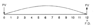
The compound-interest formula,
[latex]FV = PV(1+i)^n[/latex]
is in itself a simple equation of value, with the focal date at the nth period
Example 4.6.1
The builder's situation discussed above could be analyzed by an equation of value and corresponding cash-flow diagram, as follows:
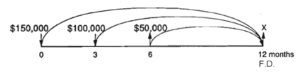
For a focal date of one year, the equation is:
[latex]\begin{align*} \text{Value of inflows} &= \text{Value of outflows}\\ (\text{FV of }$150,000)+(\text{FV of }$100,000)&= (\text{FV of }$50,000) + x\\ $150,000 (1.01)^{12} + $100,000( 1.01)^9 &=$50,000( 1.01)^6 + x\\ $169,023.75+ $109,368.53&=$53,076.01+x\\ $278,392.28-$53,076.01&=x\\ x &=$225,316.27 \end{align*}[/latex]
Through the example above, you will appreciate that the equation of value allows for the same interest as the account method does. This is true no matter what focal date is chosen - which is not the case in Simple Interest.
Since the time of the last flow was chosen as the focal date, all flows are evaluated by future value. Any cash flow that precedes the focal date is evaluated by finding its future value. Any cash flow that follows the focal date is evaluated by finding its present value.
To see how that works, study the next example, which uses a focal date of three months for the problem above.
Example 4.6.2
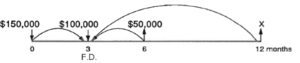
[latex]\begin{align*} \text{Value of inflows} &= \text{Value of outflows}\\ (\text{FV of }$150,000)+$100,000&=(\text{PV of }$50,000) + (\text{PV of }x)\\ $150,000.00(1.01)^3+$100,000&=\frac{$50,000}{1.01^3} +\frac{x}{1.01^9} \\ $154,545.15+$100,000&=$48,529.51+\frac{x}{1.01^9} \\ $254,545.15-$448,529.52&=\frac{x}{1.01^9} \\ x&=1.01^9 ($206,015.64)\\ x&=$225,316.27\\ \end{align*}[/latex]
This is the same answer as that obtained before, but stating and solving the equation are slightly more complex. Choosing the best focal date is a matter of convenience.
Problems may have several unknown cash flows, but it must be possible to state them in terms of one variable, since there is only one equation.
Example 4.6.3
As an example, suppose, in the builder's case, the loans were to be repaid with two equal-sized payments: one at six months, the other at one year.
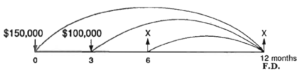
The equation is simplest if you choose one year as the focal date.
Then:
[latex]\begin{align*} \text{Value of inflows} &= \text{Value of outflows}\\ (\text{FV of }$150,000)+(\text{FV of }$100,000)&=(\text{FV of }x)+x\\ $150,000(1.01)^{12} +$100,000 (1.01)^9&= x(1.01)^6 + x\\ $169,023.75+$109,368.53 &= 1.061520151x + x\\ \frac{$278,392.28}{2.061520151} &= x\\ x&=$135,042.23 \end{align*}[/latex]
To check that this is correct, enter the values in an account as shown in the box:
| Time (months) | Interest | Cash Flow | Balance |
| 0 | $150,000 | $150,000 | |
| 3 | [latex]$150,000(1.01)^3=$154,545.15[/latex] | 100,000.00 | 254,545.15 |
| 6 | [latex]$254,545.15(1.01)^3=$262,258.12[/latex] | -135,042.23 | 127,215.89 |
| 12 | [latex]$127,215.89(1.01)^6=$135,042.23[/latex] | -135,042.23 | 0 |
It is easy to check results by an account, but it would be difficult to solve such a problem by an account. And in this case an equation would have to be solved at some point.
Your Own Notes
- Are there any notes you want to take from this section? Is there anything you'd like to copy and paste below?
- These notes are for you only (they will not be stored anywhere)
- Make sure to download them at the end to use as a reference
