2.2 Linear Functions
Tables give the values immediately, without calculation, but they may have to be very large to be useful. (Clearly the small table used in Example 2.1.1 is not large enough to be of real use in a business.) Tables are still commonly used in some areas of business - for example, to find the payments required for loans such as mortgages. They are useful because the calculations are fairly complicated and a precise answer is required. Later chapters deal with such payments. Normally we use spreadsheet programs such as Microsoft Excel for this type of problem.
Graphs communicate an overall understanding of the way a function behaves. Complex functions are often referred to by graphs. The function values and equations may not be known in detail, and the general behavior of the function may be all that is required. In economics, for example, the major issue may be the direction (up or down) that changes in one variable (such as price) have on another variable (such as revenue).
The rest of this chapter examines a type of function often used in industry and finance: linear functions.
A function is linear if the graph of the function forms a straight line. You will get a straight-line graph if the only operations on the independent variable are as follows:
- The independent variable is multiplied by a constant. For example, [latex]S= 1.4C[/latex]; Or
- The independent variable is added to or subtracted from a constant. For example, [latex]y= x+4[/latex]; Or
- A combination of 1 and 2 is used. For example, [latex]t=5+2n[/latex]
All of the above would qualify as linear functions. Note that direct variation is a special case of linear function.
The following equations would result in non-linear functions:
[latex]y=x^2-7\:\:(a\:parabola)[/latex]
[latex]v=4+\frac{2}{n}\:\:(a\: hyperbola)[/latex]
Example 2.2.1
Take the cost of producing advertising posters as an example of applying a linear function. Suppose that the management of the print shop finds that producing the posters for local companies costs $80.00 for artwork and set-up, and an additional $0.11 for materials and labor for each poster printed.
The cost of production could be described by the (linear) equation
[latex]C = 80 + 0.11x[/latex]
where
- C is the cost of production and
- x is the number of posters produced
| Number Of | ||
| Posters | Cost | |
| 100 | $ 91.00 | This table would be satisfactory |
| 200 | 102.00 | for costing orders to the printer |
| 300 | 113.00 | as long as orders were limited |
| 400 | 124.00 | to these sizes. |
| 500 | 135.00 | |
| 600 | 146.00 | |
| 700 | 157.00 | |
| 800 | 168.00 | |
| 900 | 179.00 | |
| 1,000 | 190 .00 |
To make a graph showing this function you should take as a horizontal axis the independent variable x (number of posters), and as a vertical axis the dependent variable C (cost). Both axes must be scaled so as to allow for the largest value of each variable (2,000 for x , $300 for C). Plotting the points from the table above, you get, by joining them, the graph illustrated below.
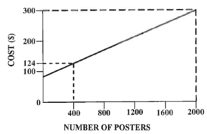
The values corresponding to a few points have been marked on the graph and dotted lines given to show how these points relate to the axes. Note that the graph is a straight line.
All linear functions are quite simple: only two points are necessary to establish the appearance of the function. An extra point serves as a check to see that the graph is correct.
Key Takeaways
Also note that as the independent variable (number of posters) increases, the dependent variable (cost) increases at a steady rate ($0.11 per poster).
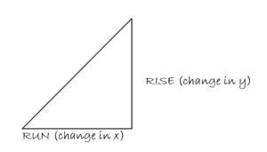
The key fact about linear functions is this uniform rate of change, which is called the slope of the line. If you revert to the generally used and for independent and dependent variables.
Then,
[latex]slope = \frac{rise}{run} = \frac{\text{change in }y}{\text{change in }x}[/latex]
= change in y per unit change of x
The slope will always have the value of the coefficient (multiplier) of if y is written as a function of x.
Thus,
[latex]y = a+bx[/latex]
Where,
- a and b are constants.
- a is the y-intercept ( y-value at = 0).
- b is the slope of the line.
Key Takeaway
Example 2.2.2
As an example, suppose you have the following linear function:
[latex]y = 3+2x[/latex]
Then the slope will have the value +2. Make a table of a few values and graph the function. Just substitute selected values of x to get values of y.
For example, if [latex]x = -2[/latex]:
[latex]3=2x=3+2(-2)=3-4=-1[/latex]
| x | y |
| -2 | -1 |
| -1 | 1 |
| 0 | 3 |
| 4 | 11 |
Key Takeaways
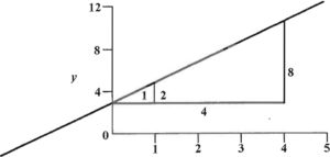
- When x changes by 1, y changes by 2.
- When x changes by 4, y changes by 2 × 4 = 8.
- Also [latex]a= 3[/latex] is the value of y when [latex]x= 0[/latex].
The graph would then appear as shown in Figure 2:
Knowledge Check 2.1
- For each of the following linear equations find the intercept and the slope.
- [latex]y = 6+3x[/latex]
- [latex]t = 2n+4[/latex]
- [latex]5s = 10-5r[/latex]
- A machine that wraps boxes of candy requires 90 minutes to set up, then one-half minute per box to do the wrapping. Use T = total time required (in minutes) x = number of boxes to be wrapped.
- Complete the equation for T. Note the units used.
Total time = set up time + wrapping time.[latex]T(min) = \_\_\_ \times \_\_\_\frac{minutes}{box}\times x \; boxes[/latex]without units:[latex]T(min) =\_\_\_\times \_\_\_\frac{minutes}{box}\times x \; boxes[/latex] - Complete the table for the given x-values:
x T 0 80 150 - Plot the points from your table on the graph and join them to form a line.

- Estimate the time to wrap 100 bags and check by calculating it with the function.
- Complete the equation for T. Note the units used.
Linear Equations from Data
You will not always be given the equation for a linear function. Instead you will have available some information about it and, from that data, you will have to work out the equation.
The most common case is to have two data points, [latex](x_1, y_1)[/latex] and [latex](x_2,y_2)[/latex] which satisfy the equation. Then, since you are working with the slope-intercept form of linear equation, you should first work out the slope, b, as follows:
[latex]Slope = b = \frac{rise}{run} = \frac{y_2-y_1}{x_2-x_1}[/latex]
Next, substitute one data point, say [latex](x_1, y_1)[/latex] into the equation to find the intercept, a, as follows:
[latex]y_1 = a+bx_1[/latex]
which can then be solved for the intercept as it is the only unknown.
Example 2.2.3
Suppose that in the poster printing example above you were only given the facts that, to make 1,000 posters, it would cost $190 and, to make 1,500 posters, it would cost $245. The information could be organized by thinking of the points as being in a table or on a graph as follows:
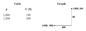
Then to find the slope:
[latex]slope=b=\frac{rise}{run}=\frac{ y_2-y_1}{x_2-x_1}=\frac{$245-$190}{1,500 -1000}=\frac{$55}{500}=$0.11\text{ per poster}[/latex]
To find the y-intercept:
[latex]$190 = a +$0.11× 1,000[/latex]
[latex]a=$190-$0.11× 1,000=$190-$110=$80[/latex]
and write the whole equation as follows:
[latex]C =$80 +$0.11x[/latex]
Knowledge Check 2.2
There are two temperature scales in North America: Fahrenheit and Celsius. They are related by a linear equation. The temperature of boiling water is 212° Fahrenheit and 100° Celsius. The temperature of freezing water is 32° Fahrenheit and 0° Celsius.
Let,
F = temperature on the Fahrenheit scale (the y).
C = temperature on the Celsius scale (the x).
Then find the equation for F in terms of C (i.e., [latex]F = a+ bC[/latex]) by using the following steps:
- Choose one point as [latex](x_1,y_1)[/latex] another as [latex](x_2,y_2)[/latex] in the formula,
[latex]slope=b=\frac{rise}{run}= \frac{y_2-y_1}{x_2-x_1 }= \frac{?}{?}= ?[/latex] - Since you now know b, substitute b and one of the known points in [latex]F =a+ bC[/latex]
and solve for a. - Write the final equation and find the Fahrenheit temperature equivalent to 20 degrees Celsius (approximately room temperature).
Your Own Notes
- Are there any notes you want to take from this section? Is there anything you'd like to copy and paste below?
- These notes are for you only (they will not be stored anywhere)
- Make sure to download them at the end to use as a reference
