Potential Energy and Conservation of Energy
Potential Energy Diagrams and Stability
Learning Objectives
By the end of this section, you will be able to:
- Create and interpret graphs of potential energy
- Explain the connection between stability and potential energy
Often, you can get a good deal of useful information about the dynamical behavior of a mechanical system just by interpreting a graph of its potential energy as a function of position, called a potential energy diagram. This is most easily accomplished for a one-dimensional system, whose potential energy can be plotted in one two-dimensional graph—for example, U(x) versus x—on a piece of paper or a computer program. For systems whose motion is in more than one dimension, the motion needs to be studied in three-dimensional space. We will simplify our procedure for one-dimensional motion only.
First, let’s look at an object, freely falling vertically, near the surface of Earth, in the absence of air resistance. The mechanical energy of the object is conserved, [latex]E=K+U,[/latex] and the potential energy, with respect to zero at ground level, is [latex]U\left(y\right)=mgy,[/latex] which is a straight line through the origin with slope [latex]mg[/latex]. In the graph shown in (Figure), the x-axis is the height above the ground y and the y-axis is the object’s energy.
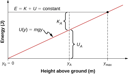
The line at energy E represents the constant mechanical energy of the object, whereas the kinetic and potential energies, [latex]{K}_{A}[/latex] and [latex]{U}_{A},[/latex] are indicated at a particular height [latex]{y}_{A}.[/latex] You can see how the total energy is divided between kinetic and potential energy as the object’s height changes. Since kinetic energy can never be negative, there is a maximum potential energy and a maximum height, which an object with the given total energy cannot exceed:
If we use the gravitational potential energy reference point of zero at [latex]{y}_{0},[/latex] we can rewrite the gravitational potential energy U as mgy. Solving for y results in
We note in this expression that the quantity of the total energy divided by the weight (mg) is located at the maximum height of the particle, or [latex]{y}_{\text{max}}.[/latex] At the maximum height, the kinetic energy and the speed are zero, so if the object were initially traveling upward, its velocity would go through zero there, and [latex]{y}_{\text{max}}[/latex] would be a turning point in the motion. At ground level, [latex]{y}_{0}=0[/latex], the potential energy is zero, and the kinetic energy and the speed are maximum:
The maximum speed [latex]\text{±}{v}_{0}[/latex] gives the initial velocity necessary to reach [latex]{y}_{\text{max}},[/latex] the maximum height, and [latex]\text{−}{v}_{0}[/latex] represents the final velocity, after falling from [latex]{y}_{\text{max}}.[/latex] You can read all this information, and more, from the potential energy diagram we have shown.
Consider a mass-spring system on a frictionless, stationary, horizontal surface, so that gravity and the normal contact force do no work and can be ignored ((Figure)). This is like a one-dimensional system, whose mechanical energy E is a constant and whose potential energy, with respect to zero energy at zero displacement from the spring’s unstretched length, [latex]x=0,\phantom{\rule{0.2em}{0ex}}\text{is}\phantom{\rule{0.2em}{0ex}}U\left(x\right)=\frac{1}{2}k{x}^{2}[/latex].
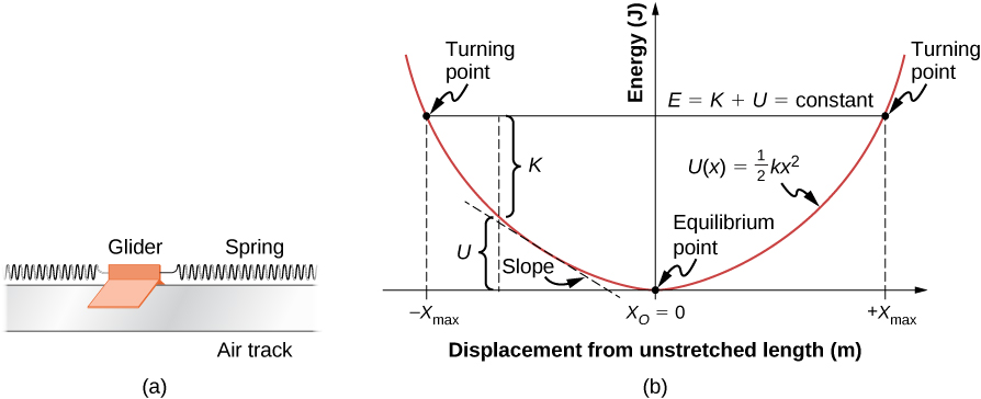
You can read off the same type of information from the potential energy diagram in this case, as in the case for the body in vertical free fall, but since the spring potential energy describes a variable force, you can learn more from this graph. As for the object in vertical free fall, you can deduce the physically allowable range of motion and the maximum values of distance and speed, from the limits on the kinetic energy, [latex]0\le K\le E.[/latex] Therefore, [latex]K=0[/latex] and [latex]U=E[/latex] at a turning point, of which there are two for the elastic spring potential energy,
The glider’s motion is confined to the region between the turning points, [latex]\text{−}{x}_{\text{max}}\le x\le {x}_{\text{max}}.[/latex] This is true for any (positive) value of E because the potential energy is unbounded with respect to x. For this reason, as well as the shape of the potential energy curve, U(x) is called an infinite potential well. At the bottom of the potential well, [latex]x=0,U=0[/latex] and the kinetic energy is a maximum, [latex]K=E,\phantom{\rule{0.2em}{0ex}}\text{so}\phantom{\rule{0.2em}{0ex}}{v}_{\text{max}}=\text{±}\sqrt{2E\text{/}m}.[/latex]
However, from the slope of this potential energy curve, you can also deduce information about the force on the glider and its acceleration. We saw earlier that the negative of the slope of the potential energy is the spring force, which in this case is also the net force, and thus is proportional to the acceleration. When [latex]x=0[/latex], the slope, the force, and the acceleration are all zero, so this is an equilibrium point. The negative of the slope, on either side of the equilibrium point, gives a force pointing back to the equilibrium point, [latex]F=\text{±}kx,[/latex] so the equilibrium is termed stable and the force is called a restoring force. This implies that U(x) has a relative minimum there. If the force on either side of an equilibrium point has a direction opposite from that direction of position change, the equilibrium is termed unstable, and this implies that U(x) has a relative maximum there.
Quartic and Quadratic Potential Energy Diagram
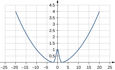
The potential energy for a particle undergoing one-dimensional motion along the x-axis is [latex]U\left(x\right)=2\left({x}^{4}-{x}^{2}\right),[/latex] where U is in joules and x is in meters. The particle is not subject to any non-conservative forces and its mechanical energy is constant at [latex]E=-0.25\phantom{\rule{0.2em}{0ex}}\text{J}[/latex]. (a) Is the motion of the particle confined to any regions on the x-axis, and if so, what are they? (b) Are there any equilibrium points, and if so, where are they and are they stable or unstable?
Strategy
First, we need to graph the potential energy as a function of x. The function is zero at the origin, becomes negative as x increases in the positive or negative directions ([latex]{x}^{2}[/latex] is larger than [latex]{x}^{4}[/latex] for [latex]x<1[/latex]), and then becomes positive at sufficiently large [latex]|x|[/latex]. Your graph should look like a double potential well, with the zeros determined by solving the equation [latex]U\left(x\right)=0[/latex], and the extremes determined by examining the first and second derivatives of U(x), as shown in (Figure).
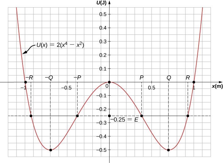
You can find the values of (a) the allowed regions along the x-axis, for the given value of the mechanical energy, from the condition that the kinetic energy can’t be negative, and (b) the equilibrium points and their stability from the properties of the force (stable for a relative minimum and unstable for a relative maximum of potential energy).
You can just eyeball the graph to reach qualitative answers to the questions in this example. That, after all, is the value of potential energy diagrams. You can see that there are two allowed regions for the motion [latex]\left(E>U\right)[/latex] and three equilibrium points (slope [latex]dU\text{/}dx=0\right),[/latex] of which the central one is unstable [latex]\left({d}^{2}U\text{/}d{x}^{2}<0\right),[/latex] and the other two are stable [latex]\left({d}^{2}U\text{/}d{x}^{2}>0\right).[/latex]
Solution
- To find the allowed regions for x, we use the condition
[latex]K=E-U=-\frac{1}{4}-2\left({x}^{4}-{x}^{2}\right)\ge 0.[/latex]
If we complete the square in [latex]{x}^{2}[/latex], this condition simplifies to [latex]2{\left({x}^{2}-\frac{1}{2}\right)}^{2}\le \frac{1}{4},[/latex] which we can solve to obtain
[latex]\frac{1}{2}-\sqrt{\frac{1}{8}}\le {x}^{2}\le \frac{1}{2}+\sqrt{\frac{1}{8}}.[/latex]This represents two allowed regions, [latex]{x}_{p}\le x\le {x}_{R}[/latex] and [latex]\text{−}{x}_{R}\le x\le -{x}_{p},[/latex] where [latex]{x}_{p}=0.38[/latex] and [latex]{x}_{R}=0.92[/latex] (in meters).
- To find the equilibrium points, we solve the equation
[latex]dU\text{/}dx=8{x}^{3}-4x=0[/latex]
and find [latex]x=0[/latex] and [latex]x=\text{±}{x}_{Q}[/latex], where [latex]{x}_{Q}=1\text{/}\sqrt{2}=0.707[/latex] (meters). The second derivative
[latex]{d}^{2}U\text{/}d{x}^{2}=24{x}^{2}-4[/latex]is negative at [latex]x=0[/latex], so that position is a relative maximum and the equilibrium there is unstable. The second derivative is positive at [latex]x=\text{±}{x}_{Q}[/latex], so these positions are relative minima and represent stable equilibria.
Significance
The particle in this example can oscillate in the allowed region about either of the two stable equilibrium points we found, but it does not have enough energy to escape from whichever potential well it happens to initially be in. The conservation of mechanical energy and the relations between kinetic energy and speed, and potential energy and force, enable you to deduce much information about the qualitative behavior of the motion of a particle, as well as some quantitative information, from a graph of its potential energy.
Check Your Understanding Repeat (Figure) when the particle’s mechanical energy is [latex]+0.25\phantom{\rule{0.2em}{0ex}}\text{J.}[/latex]
a. yes, motion confined to [latex]-1.055\phantom{\rule{0.2em}{0ex}}\text{m}\le x\le 1.055\phantom{\rule{0.2em}{0ex}}\text{m}[/latex]; b. same equilibrium points and types as in example
Before ending this section, let’s practice applying the method based on the potential energy of a particle to find its position as a function of time, for the one-dimensional, mass-spring system considered earlier in this section.
Sinusoidal Oscillations
Find x(t) for a particle moving with a constant mechanical energy [latex]E>0[/latex] and a potential energy [latex]U\left(x\right)=\frac{1}{2}k{x}^{2}[/latex], when the particle starts from rest at time [latex]t=0[/latex].
Strategy
We follow the same steps as we did in (Figure). Substitute the potential energy U into (Figure) and factor out the constants, like m or k. Integrate the function and solve the resulting expression for position, which is now a function of time.
Solution
Substitute the potential energy in (Figure) and integrate using an integral solver found on a web search:
From the initial conditions at [latex]t=0,[/latex] the initial kinetic energy is zero and the initial potential energy is [latex]\frac{1}{2}k{x}_{0}{}^{2}=E,[/latex] from which you can see that [latex]{x}_{0}\text{/}\sqrt{\left(2E\text{/}k\right)}=\text{±}1[/latex] and [latex]{\text{sin}}^{-1}\left(\text{±}\right)=\text{±}{90}^{0}.[/latex] Now you can solve for x:
Significance
A few paragraphs earlier, we referred to this mass-spring system as an example of a harmonic oscillator. Here, we anticipate that a harmonic oscillator executes sinusoidal oscillations with a maximum displacement of [latex]\sqrt{\left(2E\text{/}k\right)}[/latex] (called the amplitude) and a rate of oscillation of [latex]\left(1\text{/}2\pi \right)\sqrt{k\text{/}m}[/latex] (called the frequency). Further discussions about oscillations can be found in Oscillations.
Check Your Understanding Find [latex]x\left(t\right)[/latex] for the mass-spring system in (Figure) if the particle starts from [latex]{x}_{0}=0[/latex] at [latex]t=0.[/latex] What is the particle’s initial velocity?
[latex]x\left(t\right)=\text{±}\sqrt{\left(2E\text{/}k\right)}\phantom{\rule{0.2em}{0ex}}\text{sin}\left[\left(\sqrt{k\text{/}m}\right)t\right]\phantom{\rule{0.2em}{0ex}}\text{and}\phantom{\rule{0.2em}{0ex}}{v}_{0}=\text{±}\sqrt{\left(2E\text{/}m\right)}[/latex]
Summary
- Interpreting a one-dimensional potential energy diagram allows you to obtain qualitative, and some quantitative, information about the motion of a particle.
- At a turning point, the potential energy equals the mechanical energy and the kinetic energy is zero, indicating that the direction of the velocity reverses there.
- The negative of the slope of the potential energy curve, for a particle, equals the one-dimensional component of the conservative force on the particle. At an equilibrium point, the slope is zero and is a stable (unstable) equilibrium for a potential energy minimum (maximum).
Problems
A mysterious constant force of 10 N acts horizontally on everything. The direction of the force is found to be always pointed toward a wall in a big hall. Find the potential energy of a particle due to this force when it is at a distance x from the wall, assuming the potential energy at the wall to be zero.
10x with x-axis pointed away from the wall and origin at the wall
A single force [latex]F\left(x\right)=-4.0x[/latex] (in newtons) acts on a 1.0-kg body. When [latex]x=3.5\phantom{\rule{0.2em}{0ex}}\text{m,}[/latex] the speed of the body is 4.0 m/s. What is its speed at [latex]x=2.0\phantom{\rule{0.2em}{0ex}}\text{m?}[/latex]
A particle of mass 4.0 kg is constrained to move along the x-axis under a single force [latex]F\left(x\right)=\text{−}c{x}^{3},[/latex] where [latex]c=8.0\phantom{\rule{0.2em}{0ex}}{\text{N/m}}^{3}.[/latex] The particle’s speed at A, where [latex]{x}_{A}=1.0\phantom{\rule{0.2em}{0ex}}\text{m,}[/latex] is 6.0 m/s. What is its speed at B, where [latex]{x}_{B}=-2.0\phantom{\rule{0.2em}{0ex}}\text{m?}[/latex]
4.6 m/s
The force on a particle of mass 2.0 kg varies with position according to [latex]F\left(x\right)=-3.0{x}^{2}[/latex] (x in meters, F(x) in newtons). The particle’s velocity at [latex]x=2.0\phantom{\rule{0.2em}{0ex}}\text{m}[/latex] is 5.0 m/s. Calculate the mechanical energy of the particle using (a) the origin as the reference point and (b) [latex]x=4.0\phantom{\rule{0.2em}{0ex}}\text{m}[/latex] as the reference point. (c) Find the particle’s velocity at [latex]x=1.0\phantom{\rule{0.2em}{0ex}}\text{m}.[/latex] Do this part of the problem for each reference point.
A 4.0-kg particle moving along the x-axis is acted upon by the force whose functional form appears below. The velocity of the particle at [latex]x=0[/latex] is [latex]v=6.0\phantom{\rule{0.2em}{0ex}}\text{m/s}.[/latex] Find the particle’s speed at [latex]x=\left(\text{a}\right)2.0\phantom{\rule{0.2em}{0ex}}\text{m},\left(\text{b}\right)4.0\phantom{\rule{0.2em}{0ex}}\text{m},\left(\text{c}\right)10.0\phantom{\rule{0.2em}{0ex}}\text{m},\left(\text{d}\right)[/latex] Does the particle turn around at some point and head back toward the origin? (e) Repeat part (d) if [latex]v=2.0\phantom{\rule{0.2em}{0ex}}\text{m/s}\phantom{\rule{0.2em}{0ex}}\text{at}\phantom{\rule{0.2em}{0ex}}x=0.[/latex]
a. 5.6 m/s; b. 5.2 m/s; c. 6.4 m/s; d. no; e. yes
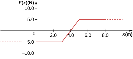
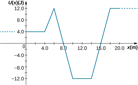
A particle of mass 0.50 kg moves along the x-axis with a potential energy whose dependence on x is shown below. (a) What is the force on the particle at [latex]x=2.0,5.0,8.0,\phantom{\rule{0.2em}{0ex}}\text{and}[/latex] 12 m? (b) If the total mechanical energy E of the particle is −6.0 J, what are the minimum and maximum positions of the particle? (c) What are these positions if [latex]E=2.0\phantom{\rule{0.2em}{0ex}}\text{J?}[/latex] (d) If [latex]E=16\phantom{\rule{0.2em}{0ex}}\text{J}[/latex], what are the speeds of the particle at the positions listed in part (a)?
(a) Sketch a graph of the potential energy function [latex]U\left(x\right)=k{x}^{2}\text{/}2+A{e}^{\text{−}\alpha {x}^{2}},[/latex] where [latex]k,A,\phantom{\rule{0.2em}{0ex}}\text{and}\phantom{\rule{0.2em}{0ex}}\alpha[/latex] are constants. (b) What is the force corresponding to this potential energy? (c) Suppose a particle of mass m moving with this potential energy has a velocity [latex]{v}_{a}[/latex] when its position is [latex]x=a[/latex]. Show that the particle does not pass through the origin unless
a. where [latex]k=0.02,A=1,\alpha =1[/latex]; b. [latex]F=kx-\alpha xA{e}^{\text{−}\alpha {x}^{2}}[/latex]; c. The potential energy at [latex]x=0[/latex] must be less than the kinetic plus potential energy at [latex]x=\text{a}[/latex] or [latex]A\le \frac{1}{2}m{v}^{2}+\frac{1}{2}k{a}^{2}+A{e}^{\text{−}\alpha {a}^{2}}.[/latex] Solving this for A matches results in the problem.
Glossary
- equilibrium point
- position where the assumed conservative, net force on a particle, given by the slope of its potential energy curve, is zero
- potential energy diagram
- graph of a particle’s potential energy as a function of position
- turning point
- position where the velocity of a particle, in one-dimensional motion, changes sign
