Appendix: Fundamental Statistics
This appendix covers the fundamental statistical concepts necessary to critically appraise randomized controlled trials (RCTs) and systematic reviews/meta-analyses.
P-Value Interpretation
P-values are sometimes misinterpreted to mean “the probability that the results occurred by chance”. This is problematic on at least two counts: the probability of any particular result occurring by chance will be extremely low, and also “by chance” requires further definition to be meaningful. A more technical definition is that the p-value is the probability of finding a result at least as extreme as the observed result if the null hypothesis (usually “no difference”) is correct and all assumptions used to compute the p-value are met.
Errors in p-value interpretation usually involve confusing the following two probabilities:
- The probability that the treatment is ineffective given the observed evidence (the misinterpretation of a p-value)
- The probability of the observed evidence if the treatment were ineffective (what the p-value provides)
- For more information on this common inference mistake (known as the “The Prosecutor’s Fallacy”) see Westreich D et al.
By convention, a p-value ≤0.05 is considered statistically significant, though this is increasingly recognized as an oversimplification and ignores consideration of clinical importance.
The most important takeaway from this discussion is that the typical understanding of a p-value is incorrect and such misunderstanding can lead to erroneous conclusions. For a further discussion of p-value misinterpretation in medical literature see Price R et al. For a more advanced discussion on why research findings are often false despite statistically significant results see Ioannidis JPA.
Confidence Interval (CI) Interpretation
The technical definition of a 95% confidence interval (CI) is: If we were to repeat the study an infinite number of times, 95% of 95% CIs would contain the true effect, if all assumptions used to calculate the interval are correct. Consequently, a 95% CI does not entail “there is a 95% chance the true value is within this range” (a common misinterpretation). As with p-values, the true meaning is more nuanced. See here for visual CI simulations as illustrative examples.
The 95% CI provides all of the information of a p-value (and is derived using the same information), but also adds information on a plausible range of the effect size. When interpreting CIs, it is important to examine both ends of the CI and judge whether there is a clinically important difference between them. For example, a point estimate of 5% absolute risk reduction in stroke risk over 5 years with a 95% CI of 3% to 7% will include a narrow range that many clinicians would consider clinically important difference at both ends of the interval. This examination (along with considerations of bias) will help establish the degree of uncertainty in the result. See McCormack J et al. for a discussion of how considering only statistical significance without proper regard for CIs can cause confusion.
By convention, a 95% CI that does not include the null (e.g. a relative effect 95% CI that includes 1.0 or an absolute risk difference 95% CI that includes 0%) is considered statistically significant (i.e. consistent with p<0.05).
Sample Size Interpretation
It is sometimes believed that sample size (i.e. how many participants were included in the study) is a determinant of internal validity. However, a review (Kjaergard LL et al.) found that smaller trials (<1,000 participants) only exaggerated treatment effects compared with larger trials (≥1,000 participants) when they had inadequate randomization, allocation concealment, or blinding. As such, sample size itself is not indicative of bias. Furthermore, if there were too few participants enrolled to detect a difference between groups this will be reflected in the corresponding wide CI (see Confidence Intervals – How precise were the estimates of treatment effect? for a discussion of wide CIs and how they illustrate precision).
Advanced discussion (included for completeness, but rarely applicable to appraisal)
An exception may be true for some “very small” trials – as parametric statistical tests rely on the central limit theorem and require a minimum sample size (e.g. n≥30 is often suggested). See Fagerland MW for a more discussion. The details of this particular statistical concern are beyond the scope of this resource, but two simplified takeaways are that:
- “Very small” sample size may be a concern for the proper use of certain statistical methods when measuring continuous outcomes
- A minimum sample of 30 is an arbitrary rule-of-thumb to prevent this – nonetheless 30 does provide an approximation of the sample sizes where this may be a concern (e.g. this will almost certainly not be a concern for a trial with several hundreds of participants)
Absolute Risk Differences and Relative Measures of Effect
Absolute Risk Difference
The absolute risk difference between groups refers to the risk of an event in one group minus the risk in another group. Consider the following example of a theoretical 2 year trial examining insomnia rates:
| Outcome | Intervention Group | Comparator Group | Absolute Difference | Duration |
| Insomnia | 15% | 5% | +10% | 2 years |
In this case, the absolute difference was calculated by subtracting the intervention group event rate (15%) by the comparator group event rate (5%), which equals 10% (15% – 5%). This difference is “absolute” because the number (e.g. +10% risk of insomnia over 2 years) is independently meaningful.
Absolute differences also need to be communicated in the context of time. For example, a 1% absolute risk reduction over 1 month is quite different from a 1% absolute risk reduction over 10 years. As such, absolute differences should be stated as a __% increase/decrease over [timeframe].
Relative Measures of Effect
This contrasts with relative effect measures. One example of a relative effect is relative risk (RR), which is calculated by dividing the risk of event in the intervention group by that in the comparator group.
| Outcome | Intervention Group | Comparator Group | Relative Risk (RR) | Duration |
| Insomnia | 15% | 5% | 3.0 | 3 months |
In this case, the RR was calculated by dividing the intervention group rate (15%) by the comparator group event rate (5%), which equals 3.0 (15% ÷ 5%). This difference is “relative” because the number (e.g. a 3.0 RR of experiencing insomnia) is dependent on the risk in the comparator group to be meaningful. RR 3.0 means that the risk has tripled, but without knowing the baseline risk that is being tripled, then the number is not fully interpretable.
This dependence can be problematic if not properly considered. Consider the following example, where the RR is identical in both cases:
| Relative Risk (RR) | Baseline Risk | Risk on Treatment (RR x Baseline Risk) |
Absolute Risk Difference | Duration |
| 0.5 | 30% | 15% | 15% | 10 years |
| 0.5 | 2% | 1% | 1% | 10 years |
As demonstrated, RR considered in isolation lacks crucial information. The same concept is relevant when (responsibly) buying a product during a sale. Knowing that a particular product is 50% off is not sufficient for a rational choice, as there needs to also be information about the original price (e.g. $20 versus $20,000) before deciding if the purchase is desirable.
Note: RR is just one relative measure – see discussion below for information on relative risks, odds ratios, and hazard ratios.
Number Needed to Treat or Harm
Both number needed to treat (NNT) and number needed to harm (NNH) are measures of how many patients have to receive the treatment of interest for one additional person to experience the outcome of interest (NNT being for beneficial outcomes, and NNH for harmful outcomes).
It is calculated as: 100 ÷ Absolute risk difference, with the result always rounded up.
For example, if a treatment has a 7% absolute risk increase of causing urinary retention over 3 months then the NNH is 15 (100 ÷ 7 = 14.3, then round up to 15). This means that 15 patients will have to be treated for one of them to have urinary retention over the next 3 months (always including timeframe, as with absolute risk differences).
This is an alternative way to understand absolute risk differences that may be more intuitive to some (though it is more poorly understood by patients than other measures, as discussed here).
Relative Risk, Odds Ratios, and Hazard Ratios
Before delving into the details of each type of relative effect it should be noted that all of them have the following features:
Any relative measure = 1.0 means there was no difference between groups
Any relative measure > 1.0 means the outcome was more likely with the intervention than the comparator
Any relative measure < 1.0 means the outcome was less likely with the intervention than the comparator
To demonstrate the differences between these measures of relative effect, consider the following table:
| Stroke | No stroke | |
| Aspirin | 10 (A) | 90 (B) |
| Placebo | 20 (C) | 80 (C) |
Relative Risk (RR)
Calculating the RR consists of dividing the risk of event in the aspirin group by risk of event in the placebo group.
Using the above table:
The risk of event in the treatment group: A ÷ (A+B)
The risk of event in the comparator group: C ÷ (C+D)
With numbers imputed: 10 ÷ 100 = 0.1 (or 10%) in the aspirin group and 20 ÷ 100 = 0.2 (or 20%) in the placebo group.
The RR is then 0.1 ÷ 0.2 = 0.5.
Odds Ratio (OR)
Calculating the OR consists of dividing the odds of an event in the aspirin group by the odds of an event in the placebo group.
Using the above table:
The odds of event in intervention group: A ÷ B
The odds of event in the comparator group: C ÷ D
With numbers imputed: 10 ÷ 90 = 0.11 in the aspirin group and 20 ÷ 80 = 0.25 in the placebo group.
The OR is then 0.11 ÷ 0.25 = 0.44.
OR are similar to RR when events are rare (A ÷ (A+B) ≈ A ÷ B when A is very small) (Holcomb WL et al.). As events become more common, these measures diverge and ORs will overestimate RRs (such as in this example where RR=0.5 and OR=0.44). The ClinCalc tool can be used to convert OR to RR.
Hazard Ratio (HR)
Hazard ratios (HRs) represent the average of the instantaneous incidence rate at every point during a trial. Consider an example of a 5-year trial that has a HR of 0.70 for the outcome of death comparing an intervention against some comparator. This means that a participant assigned to intervention will be 30% less likely to die relative to the comparator at any point during the trial:
- Year 1: If 5% have died in the comparator group, then 3.5% are expected to have died in the intervention group (5% * 0.70 = 3.5%)
- Year 2: If 10% have died in the comparator group, then 7% are expected to have died in the intervention group (10% * 0.70 = 7%)
- Year 5: If 20% have died in the comparator group, 14% are expected to have died in the intervention group (20% * 0.70 = 14%)
The same is approximately true at any given timepoint during the trial follow-up. These are all approximations as the HR is an average, it (almost certainly) will not be exactly true at every time point. For instance, the final HR might be 0.70, but it could be 0.80 during the first half of the trial and 0.60 during the latter half.
For example, consider the unadjusted analysis from an observational study (Turgeon RD, Koshman SL, et al.) that compared the use of ticagrelor vs. clopidogrel in patients who had undergone percutaneous coronary intervention following acute coronary syndrome (ACS). For the outcome of survival without major adverse coronary events (MACE) the HR was 0.84 before adjustment for potential confounding variables, depicted visually below:
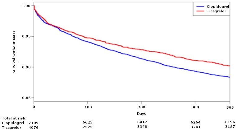
Graph 3. Kaplan Meier curve of survival without major adverse coronary events
While not exactly true at every time point, past the first 100 days the cumulative proportion patients experiencing death or MACE in the ticagrelor group appears to be roughly 84% of the cumulative proportion in the clopidogrel group fairly consistently (see “Kaplan Meier Curves” for more information below on how to interpret these types of graphs). This coheres with the HR of 0.84 discussed above.
HRs are usually similar to RRs (Sutradhar R et al.). HRs examine multiple timepoints over trial follow-up, whereas RRs evaluate cumulative proportions at the end of the trial (or at another single timepoint). HRs can account for differential follow-up times, and contain more information than RRs/ORs since they include the added dimension of time (Guyatt G et al.). HRs are limited in their ability to convey fluctuations in effect over time, as a HR of 1.0 could mean that there was consistently no effect, or it could mean that there was beneficial effect during the first half and a proportional detrimental effect during the latter half (Hernán MA). However, some of these limitations can be overcome by combining a HR with the use of a Kaplan Meier curve, as discussed below.
Kaplan Meier Curves
Cumulative Hazards
Kaplan Meier curves are graphical representations comparing event accrual between two groups over time. Consider another example from the aforementioned study comparing ticagrelor vs. clopidogrel:
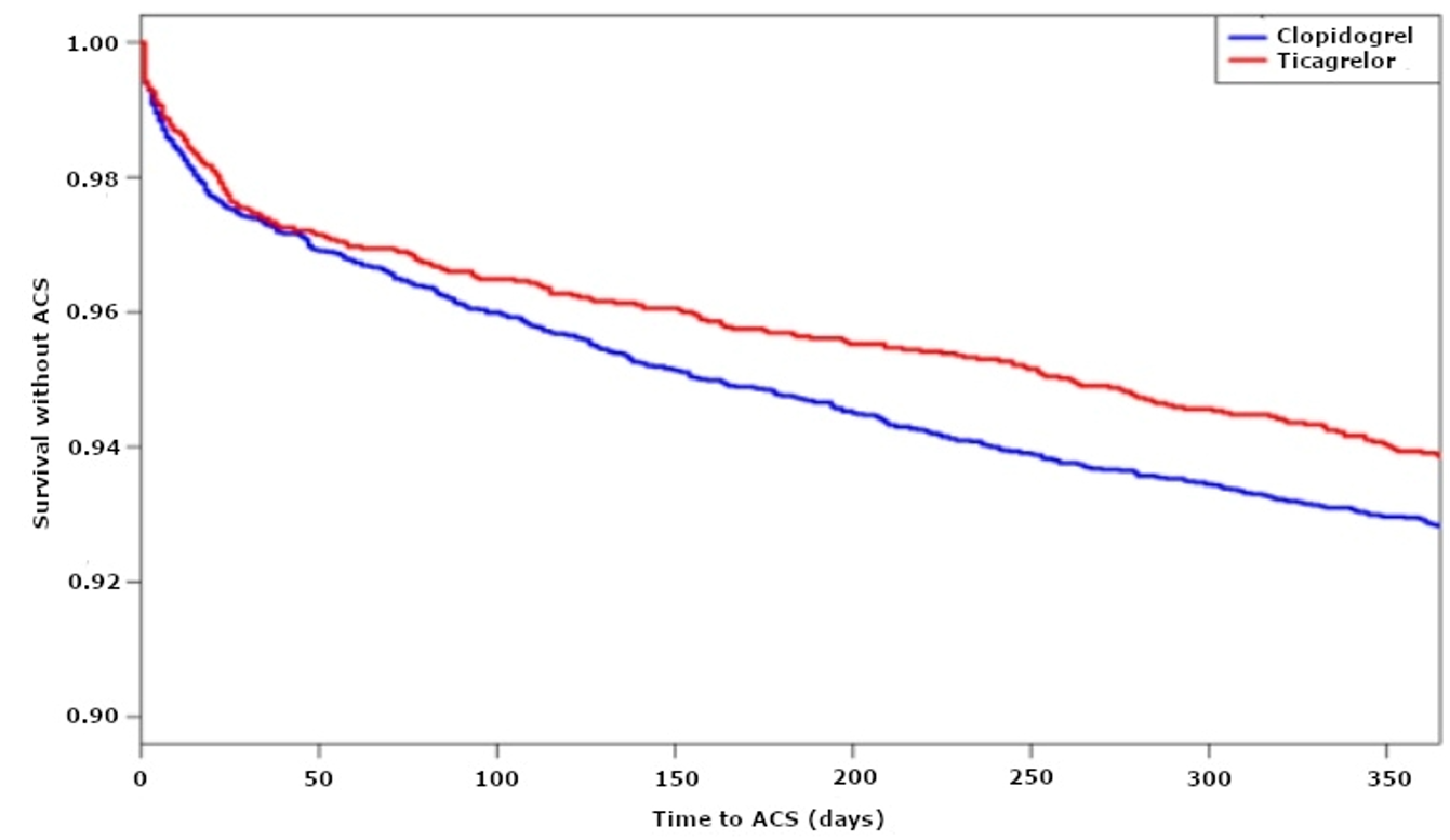
Graph 4. Kaplan Meier curve of survival without acute coronary syndrome (ACS)
Each curve displays the cumulative proportion of patients in that group who have experienced the outcome of interest. As time passes more participants experience the outcome and the curve progresses downwards. The relative differences in outcome accumulation can be expressed as a HR, as discussed above. Note that, while not displayed, each curve has a CI surrounding it at every time point.
Onset of Benefit
Consider the above Kaplan Meier curve. During the first 50 days, the curves for the two groups overlap. However, after this point the two curves begin to separate. This curve provides insight into the onset of benefit of the intervention and if the benefit is sustained over time. In this case, onset of benefit begins after approximately 50 days and is sustained as time elapses.
Course of Condition
The graph also gives insight into event rates over time. As can be seen above, the curve is steepest initially – indicating that the risk of death or ACS is highest immediately following the intervention. The slope of the curve then flattens and remains relatively stable – indicating the event rate after the initial period is relatively constant during the first year. This demonstrates how Kaplan Meier curves can be useful to understand the course of a condition over time.
Total at Risk (or Number at Risk)
Consider another curve from the same study, this one examining survival without major bleeds:
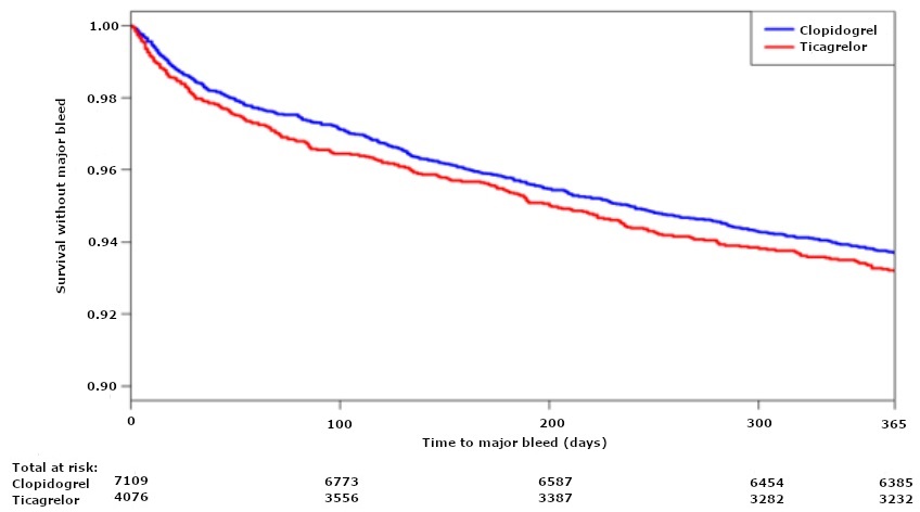
Graph 5. Kaplan Meier curve of survival without major bleeding
As depicted, sometimes there is also a “Total at risk” (sometimes called “Number at risk”) table beneath the curve. This can give additional information regarding the participants as they progressed through the trial. All participants begin “at risk”, but as the study progresses the number decreases. Below are the following reasons the number may decrease, as well as possible implications if the decreases are not balanced between groups:
| Reasons for total at risk decreasing | Implications if imbalanced between groups |
| Outcome of interest occurred | If there is a difference in effect between the intervention and comparator, then the total at risk may decrease more quickly in one group. This is evidence of effect, not bias. |
| Death | If there are differences in mortality rates then this should prompt consideration of the relative safety of the comparators, as well as consideration of death as a competing event within the analysis. |
| Loss to follow-up | This could result in systematic bias if the reasons for loss to follow-up are not random (for more see the discussion on loss to follow-up here). |
| The study ended before the participant had outcome data at that time point | If by chance there is a difference in how many patients were enrolled early in one group (and thus had more time to accrue events) this could bias a RR or OR. For example, by chance one group might have patients enrolled for an average of 4 years and another group had patients enrolled for an average of 5 years. However, since the HR incorporates the timing of events, this should not result in bias. |
Thus the total at risk table can serve as a clue that further examination should be undertaken to see if there is bias.
Forest Plots
Forest plots are used in meta-analyses to graphically depict the effects of an intervention across multiple studies. Consider the labeled example below from the “Beta-blockers for hypertension” Cochrane Review (Wiysonge CS et al.):
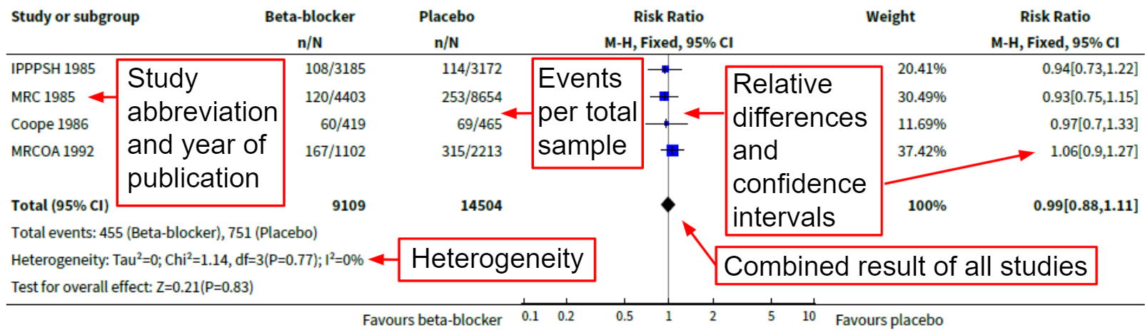 Plot 4. Forest plot of beta-blockers vs. placebo in patients with hypertension for the outcome of mortality.
As showcased, forest plots show information about each individual study included for that outcome, and also the combined results. This information is displayed visually as well as numerically. Trials with more events or participants are generally given greater weight. Heterogeneity is typically measured via I2, which is 0% in this case. For more information on heterogeneity see here.
Standardized Mean Difference Interpretation
The standardized mean difference (SMD) is a method of combining multiple continuous outcome scoring systems into one measurement. For example, when performing a meta-analysis on the effects of antidepressants on depression symptom reduction, trials may use different scales to rate depression symptoms (HAM-D, PHQ-9, etc.). SMD will allow the aggregation of the results of all these studies. Notably, using SMD assumes that differences between studies are due to differences in scales (and not in intervention/population characteristics). Arbitrary “rule-of-thumb” cutoffs (e.g. SMD of 0.2 = “small effect”) may not reflect the minimal important difference.
An alternative approach is to transform the SMD into a more familiar scale (Higgins JPT et al.). Multiply the SMD by the standard deviation (SD) of the largest trial to convert to its scale.
E.g. These are the results of a meta-analysis which assesses the effects of IV iron on health-related quality of life at 6 months in patients with HFrEF (Turgeon RD, Barry AR, et al.):
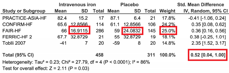
Plot 5. Forest plot of IV iron vs. placebo in patients with heart failure with reduced ejection fraction on health-related quality of life.
Step 1: Identify the trial with the most weight, FAIR-HF in this case.
Step 2: Calculate average SD. Average SD in this case is ~20.50 (the average of 16.9115 and 24.0832).
Step 3: Multiply average SD by SMD. In this case this gives 10.66 (20.50 * 0.52).
Step 4: Contextualize this result in the scale used in the trial. In this case, that would be equal to a 10.66 out of 100 improvement at 6 months (per the scale used in FAIR-HF).
Step 5: Compare this value to the minimally important difference (MID) if known. In the case of the FAIR-HF scale the MID was 5. Therefore the mean effect was greater than the MID.
Ideally the review will present this information along with a comparison of the proportion of participants within each group who experienced clinically important improvement or decline (the so-called “responder analysis”). This is useful because calculating the mean alone will not provide any information about the distribution. The responder analysis unfortunately cannot typically be calculated by readers if it is not already reported by the reviewers.
Statistical Significance Is Not Everything
While this section has focused on statistical fundamentals it is important to emphasize that statistics are only one aspect of critical appraisal. Even if a study shows statistical significance, there needs to be considerations of bias, clinical significance, and generalizability.
Bias: P-values and CIs are contingent on all the assumptions being used to calculate them being correct. In other words, they assume there is absolutely no bias present. As such, if the study is poorly conducted (e.g. a RCT without adequate allocation concealment and blinding) this will not be reflected in the statistical analysis of the results. This is why it is necessary to appraise the conduct of the trial to evaluate the credibility of the results.
Clinical significance: Even if a result is statistically significant, it may be too small of an effect to matter to a patient. For instance, with enough participants, a 1-point reduction in pain on a 100-point scale could be statistically significant, but very unlikely to be felt by an individual patient.
Generalizability: Even if the results are unbiased and clinically significant, they will only be useful if they can be applied to practice. If there are substantial differences between the features of the trial and your own practice, then the result may not be applicable.
Other sections of this resource will go into these concepts in more depth, but these are the fundamental reasons why a comprehensive approach to appraisal is necessary, and simply looking at statistical significance in the results section will not be sufficient to understand the clinical implications of a trial.
Randomized controlled trials are those in which participants are randomly allocated to two or more groups which are given different treatments.
A review that systematically identifies all potentially relevant studies on a research question. The aggregate of studies is then evaluated with respect to factors such as risk of bias of individual studies or heterogeneity among results. The qualitative combination of results is a systematic review.
A meta-analysis is a quantitative combination of the data obtained in a systematic review.
In superiority analyses, this is the hypothesis that there is no difference in the outcome of interest between the intervention group and the comparator group. In non-inferiority analyses, this is the hypothesis that there is a difference in the outcomes of interest between the treatment group and the control group.
Relative risk (or risk ratio) is the risk in one group relative to (divided by) risk in another group. For example, if 10% in the treatment group and 20% in the placebo group have the outcome of interest, the relative risk in the treatment group is 0.5 (10% ÷ 20%; half) the risk in the placebo group. See here for a more detailed discussion.
Absolute risk difference is the risk in one group compared to (minus) the risk in another group over a specified period of time. For example, if the absolute risk of myocardial infarction over 5 years was 15% for the comparator and 10% for the intervention, then the absolute risk difference was 5% (15% - 10%) over 5 years. See here for further discussion.
Systematic deviation of an estimate from the truth (either an overestimation or underestimation) caused by a study design or conduct feature. See the Catalog of Bias for specific biases, explanations, and examples.
Calculates the effect of an intervention via a fractional comparison with the comparator group (i.e. intervention group measure ÷ comparator group measure). Used for binary outcomes. Relative risk, odds ratio, or hazards ratio are all expressions of relative effect. For example, if the risk of developing neuropathy was 1% in the treatment group and 2% in the comparator group, then the relative risk is 0.5 (1 ÷ 2). See the Absolute Risk Differences and Relative Measures of Effect discussion here for more information.
The extent to which the study results are attributable to the intervention and not to bias. If internal validity is high, there is high confidence that the results are due to the effects of treatment (with low internal validity entailing low confidence).
Refers to the process that prevents patients, clinicians, and researchers from predicting which intervention group the patient will be assigned. This is different from blinding; allocation concealment refers to patients/clinicians/outcome assessors/etc. being unaware of group allocation prior to randomization, whereas blinding refers to remaining unaware of group allocation after randomization. Allocation concealment is a necessary condition for blinding. It is always feasible to implement.
Odds ratios are the ratio of odds (events divided by non-events) in the intervention group to the odds in the comparator group. For example, if the odds of an event in the treatment group is 0.2 and the odds in the comparator group is 0.1, then the OR is 2 (0.2/0.1). See here for a more detailed discussion.
Hazard ratios are a relative measure of effect. Hazards refer to average instantaneous incidence rate at every point during the trial. This differentiates it from other measures, such as relative risk, which rely only on cumulative event rates. See here for a more detailed discussion.
Loss to follow-up may occur when participants stop coming to study follow-up visits, do not answer follow-up phone calls, and cannot otherwise be assessed for study outcomes. This leads to missing data from the time they became "lost". Underlying reasons may include leaving the trial without informing investigators, moving to a new location, debilitation due to illness, or death.
Refers to variability between studies in a systematic review. It can refer to clinical differences, methodological differences, or variable results between studies. Heterogeneity occurs on a continuum and, in the case of heterogeneity amongst results, can be expressed numerically via measures of statistical heterogeneity. See here for a further discussion of statistical heterogeneity.
Transformation of continuous data that consists of dividing the difference in means between two groups by the standard deviation of the variable. In clinical research, this is often used to summarize and/or pool continuous outcomes that are measured in several ways. For example, a meta-analysis of antidepressants may need to use the SMD if trials used different scales (e.g. Beck Depression Inventory, Hamilton Depression Rating Scale) to report change in depression symptoms. See here for further discussion on SMD interpretation.
The minimum difference in a value that would be of importance to a patient. There are various methods of calculating a minimally important difference.
Refers to the extent to which the trial results are applicable beyond the patients included in the study. Also known as external validity.
