Video#1: An overview and the definition of ecological models:

Video#2: Types of ecological models:

Video#3: Some important process-based ecological models:

Contents

1 Overview
1.1 definition
1.2 Model building
1.3 Model applications
2 Types of models
2.1 Analytic models
2.2 Simulation models
2.3 Empirical and process-based models in climate change applications
3 Model building
3.1 Model design
3.2 Model validation
4 Process-based models
4.1 3-PG
4.2 FORECAST
4.3 Tree and Stand Simulator (TASS)
4.4 LANDIS-II

1 Overview

The impacts of climate change on forest ecosystems are likely to compromise tree growth, increase vulnerability to disturbances, and eventually shift in species distributions. Thus, it is likely to require changes in forest planning and natural resource management to mitigate and adapt to climate change. Ecosystem models have widely been used to understand the relationships between ecosystem and environmental conditions, and to provide a “best estimate” about how forests might work in the future and thus guide decision‐making in forest resources management.

1.1 Definition

An ecosystem model, also called an ecological model, is usually a mathematical representation of an ecological system. It is a simplified form of a highly complex ecosystem in the real world. The ecological system can range in scale from an individual population to an ecological community, or even an entire biome.

1.2 Model building

Based on data gathered from the field, ecological relationships—such as the relation of sunlight and water availability to photosynthetic rate, or frost resistance to cold temperature and the length of growth period—are derived, and these are combined to form ecosystem models.

Due to the complexity of ecosystems, it is impossible to capture every possible element of a system in a model. Thus, modelers need to take decisions about which of its features to include and which to disregard. These decisions are usually guided by the aims that the modeler is attempting to achieve. It is desirable to make an ecological model to be general (the model can be applied to a wide range of real-life systems), realistic (the model’s conclusions have a close match to a real-life system) and precise (the model’s predictions for a specific set of circumstances have little or no uncertainty). Trading-off one desideratum in order to achieve greater performance in the other two is often involved in model-building processes.

1.3 Model applications

Ecological models enable researchers to simulate large-scale experiments that would be too costly or unethical to perform on a real ecosystem. They also enable the simulation of ecological processes over very long periods of time (i.e., simulating a process that takes centuries in reality, can be done in a matter of minutes in a computer model). More importantly, ecological models can be used to predict the state of ecosystems under future climates.

Ecosystem models have applications in a wide variety of disciplines, such as natural resource management, ecotoxicology, and environmental health, agriculture, and wildlife conservation. Applications of ecological models in forest resources management to mitigate the negative impact of climate change and help forest trees to adapt to a rapidly changing environment have become particularly important.

At present, our understanding of the relationships ecosystems and the changing environment is relatively weak. The vulnerability of ecological systems, and the services provided by them, to the impact arising from climate change remain largely unknown. Ecological models have been widely used to assess the impact of climate change in terms of productivity, carbon storage, and vulnerability to disturbances, and to provide information for developing forest adaptive strategies, such as assisted migration at the species level and assisted gene-flow at the population level.

2. Types of models

There are two major types of ecological models:

1) Analytic models and

2) Simulation models.

2.1 Analytic models

Analytic models are typically relatively simple (often linear) systems, that can be accurately described by a set of mathematical equations whose behavior is well-known. Analytic models are also called correlative models or empirical models.

For example,

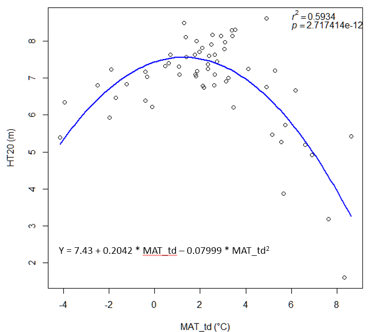
A model of tree height growth of populations originated from different climates that assumes the transfer distance of populations affects the tree height growth in a quadratic relationship as:

Y = b0 + b1 * MAT_td + b2 * MAT_td^2

Where Y is the tree height; MAT_td is the transfer distance in term of mean annual temperature; MAT_td^2 is the quadratic form of the transfer distance; and b0, b1, and b2 are parameters to be determined during the model fitting process.

A model can be acceptable if the amount of variance explained by the model is high (or the relationship is strong) based on the statistical significance (P < 0.05), such as the one illustrated in Figure 1.

Although the solution to the above simple question is fairly transparent, analytical models describing more complex systems can often become fairly complicated. However, for those comfortable with mathematics, an analytical solution does provide a concise preview of a model’s behavior that is not as readily available with a simulation model. We will focus on this type of models in this course, and more details on analytic or empirical models will come in later lectures.

2.2 Simulation models

Simulation models use numerical techniques to solve problems for which analytic models are impractical or impossible. They are also called numerical models or process-based models. A simulation model approach focuses on simulating detailed physical or biological processes that explicitly describe the behavior of a system.

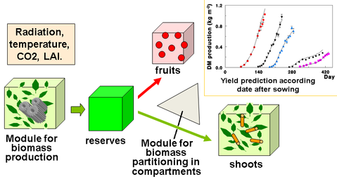
As the name stated, a process-based model can simulate the process or dynamics over time. For example, many process-based models can simulate the tree growth from seedlings to harvest, or simulate the stand performance over rotations.

2.3 Empirical and process-based models in climate change applications

Both of Empirical and process-based models are applied in modeling the impact of climate change on species distributions, productivity, and vulnerability to stress.

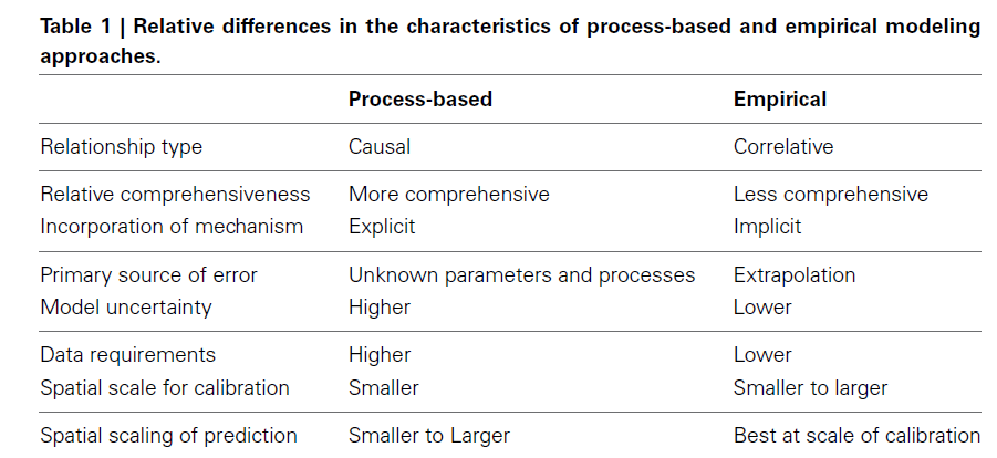
The empirical approach relies on correlative relationships in line with mechanistic understanding, but without fully describing system behaviors and interactions. For example, the model represents the relationship between the transfer distance and tree height of populations. We can see that a strong relationship is represented by the model, but the model does not show the physiological process driving this relationship.

The process-based models, on the other hand, can be more comprehensive and incorporate mechanisms explicitly. For example, many process-based models include the process of how radiation, water, and temperature affect the rate of photosynthesis, and how the biomass generated from the photosynthesis allocates to different parts of the plants, as shown in Figure 2. However, the accuracy of the model predictions is often lower than an empirical model.  This is because there are many factors affecting the performance of trees, populations, or an entire ecosystem, and many of them cannot be incorporated into the process-based model.

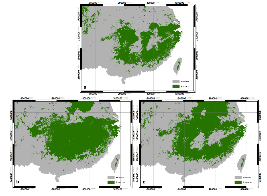
Empirical models based on the occurrence data of a species, particularly with machine-learning algorithms, have demonstrated clear superiority over process-based models in predictions of species distributions. These models are often called species distribution models (SDMs). The occurrence of the species resulted from the process of long-term local adaptation to environmental conditions, interaction with other species, and many other factors. These processes are difficult to model by a process-based model. In contrast, the empirical models do not need to consider these processes, but just relate the occurrence locations with its environmental variables. The relationships are mostly very strong. More detailed comparisons are listed in Table 1.

3. Model building

As empirical models are relatively easy to build and will be described in detail in the latter lectures; thus, this section is mostly focused on process-based models.

3.1 Model design

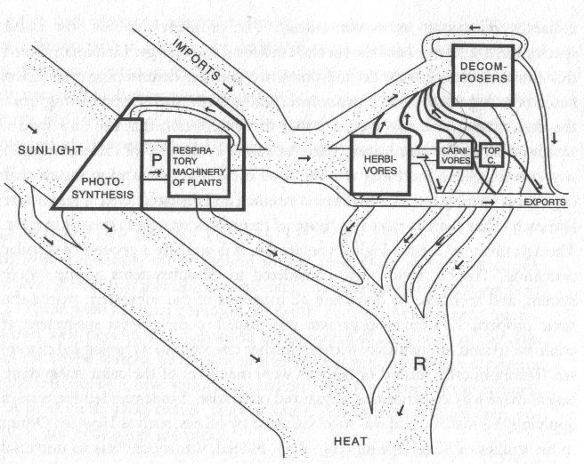
Ecological systems are composed of an enormous number of biotic and abiotic factors that interact with each other in ways that are often unpredictable, or so complex as to be impossible to incorporate into a computable model.

Because of this complexity, ecosystem models typically simplify the systems to a limited number of components that are well understood and relevant to the problem that the model is intended to solve. Thus, the process of model design needs to begin with a specification of the problem to be solved or the objectives of the model.

The process of simplification typically reduces an ecosystem to a small number of state variables and mathematical functions that describe the nature of the relationships between them. The number of ecosystem components that are incorporated into the model is limited by aggregating similar processes and entities into functional groups that are treated as a unit.

Another important factor in the ecosystem model structure is the representation of the space used. Historically, models have often ignored the confounding issue of space. However, for many ecological problems, spatial dynamics are an important part of the problem, with different spatial environments leading to very different outcomes.

Spatially explicit models (also called “spatially distributed” or “landscape” models) attempt to incorporate a heterogeneous spatial environment into the model. A spatial model is one that has one or more state variables that are a function of space or can be related to other spatial variables.

3.2 Model validation

After construction, models are validated to ensure that the results are acceptably accurate or realistic.

One method is to test the model with multiple sets of data that are independent of the actual system being studied. This is important since certain inputs can cause a faulty model to output correct results.

Another method of validation is to compare the model’s output with data collected from field observations.

Model predictions almost always involve errors. Researchers frequently specify beforehand how much of a disparity they are willing to accept between parameters output by a model and those computed from field data.

4. Process-based models

In process-based models, the environment variables and vegetation are linked up upon the comprehensive physiological processes and functions between them. They often have a high requirement for data input. The process-based approach focuses on simulating detailed physical or biological processes that explicitly describe system behavior. They can be comprehensive and mechanism explicit. All process-based models include some empirical information. Uncertainty in process-based model outputs could be higher than for the empirical approach due to greater model parameters and data inputs to represent the many processes in the system. The application of physiological rules makes process-based models possible to mimic the vegetation growth and display the future species distribution, as well as the forest dynamics.

We will introduce several process-based forest ecological models here.

4.1 3-PG

The 3-PG (Physiological Principles Predicting Growth) forest growth model has been most widely used. The 3-PG model is a simplified physiological processes-based stand growth model developed by Landsberg and Waring in 1997.

A 3-PG model calculates the radiant energy absorbed by forest canopies and converts it into biomass production. The efficiency of radiation conversion is modified by the effects of nutrition, soil drought (the model includes continuous calculation of water balance), atmospheric vapor pressure deficits, and stand age.

3-PG is a deliberate attempt to bridge the gap between conventional empirical growth and yield models, and complex process-based carbon-balance models. It can be applied to plantations, or to even-aged, relatively homogeneous forests. It is a generic stand model, in the sense that its structure is not site or species-specific. However, parameterization is necessary for improving model effectiveness when it is applied for different tree species. The 3-PG model is usually more powerful and effective after the parameter values have been adjusted for aimed tree species.

3-PG consists of five simple sub-models:

• the assimilation of carbohydrates,
• the distribution of biomass between foliage,
• roots and stems, the determination of stem number,
• soil water balance, and
• conversion of biomass into variables of interest to forest managers.

The 3-PG model has been used to stimulate forest dynamic and productivity and estimate future migration direction and distribution under changing climate. A 3-PG model can also be applied together with other tools for a more comprehensive and convincing performance.

The 3-PG model can be downloaded for free from:

https://3pg.forestry.ubc.ca/software/

4.2 FORECAST

FORECAST is a management-oriented, stand-level, forest-growth, and ecosystem-dynamics model. The model was designed to accommodate a wide variety of silvicultural and harvesting systems and natural disturbance events (e.g., fire, wind, insect epidemics) in order to compare and contrast their effect on forest productivity, stand dynamics, and a series of biophysical indicators of non-timber values. The model was developed by Kimmins and his colleagues at the University of British Columbia.

FORECAST can project stand growth and ecosystem dynamics. The projection is based upon a representation of the rates of key ecological processes regulating the availability of, and competition for, light and nutrient resources (a representation of moisture effects on soil processes, plant physiology and growth, and the consequences of moisture competition is being added).

The rates of these processes are calculated from a combination of historical bioassay data (such as biomass accumulation in plant components and changes in stand density over time) and measures of certain ecosystem variables (including decomposition rates, photosynthetic saturation curves, and plant tissue nutrient concentrations) by relating ‘biologically active’ biomass components (foliage and small roots) to calculated values of nutrient uptake, the capture of light energy, and net primary production.

Using this ‘internal calibration’ or hybrid approach, the model generates a suite of growth properties for each tree and understory plant species that is to be represented in a subsequent simulation. These growth properties are used to model growth as a function of resource availability and competition. They include (but are not limited to):

(1) photosynthetic efficiency per unit foliage biomass and its nitrogen content based on relationships between foliage nitrogen, simulated self-shading, and net primary productivity after accounting for litterfall and mortality;

(2) nutrient uptake requirements based on rates of biomass accumulation and literature- or field-based measures of nutrient concentrations in different biomass components on sites of different nutritional quality (i.e. fertility);

(3) light-related measures of the tree and branch mortality derived from stand density and live canopy height input data in combination with simulated vertical light profiles. Light levels at which mortality of branches and individual trees occur are estimated for each species.

The FORECAST model has been widely applied as a long-term management evaluation tool in a variety of forest ecosystems. The FORECAST model simulates the effect of light and nutrient availability on forest productivity but it has no explicit representation of moisture or temperature on ecosystem processes. Thus, the model is not directly driven by climate data. FORECAST Climate has been developed to incorporate these two factors. The foundation for FORECAST Climate was established through the creation of a dynamic linkage with a forest hydrology model including direct feedback to the core processes driving forest ecosystem production.

4.3 Tree & Stand Simulator (TASS)

The Tree and Stand Simulator (TASS) is a biologically based, spatially explicit, individual tree model. By simulating the potential effects of silvicultural decisions and prescriptions, TASS provides yield projections for timber supply reviews and helps resource managers identify investment opportunities. The model is developed and maintained by the Ministry of Forests, Lands, Natural Resource Ministry of Forests, Lands, Natural Resource Operations & Rural Development.

 TASS currently exists in 3 main forms:

1. TASS III is the all-new public-release Windows™ version, which begins to extend TASS into more complex stand structures with multiple-species and -age cohorts.  The initial release is limited to lodgepole pine (Pinus contorta var. latifolia) and white spruce (Picea glauca).
2. TASS II (commonly referred to as TASS) is the well-established, in-house version described below.  Although, the concepts largely apply to TASS III, as well.
3. TIPSY (Table Interpolation for Stand Yields provides direct operational access to yield tables generated by TASS II.  For scenarios outside the limited range of TIPSY, a custom TASS run service is available by contacting the Growth and Yield Application Specialist.

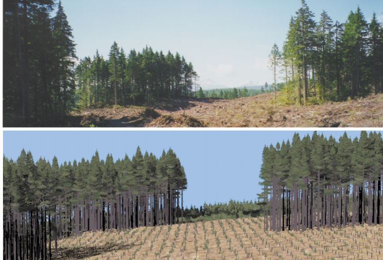
Photos in Figure 5 show trees remaining after variable retention harvesting by Weyerhaeuser Company Limited (the real world), and the TASS simulations. They are amazingly similar.

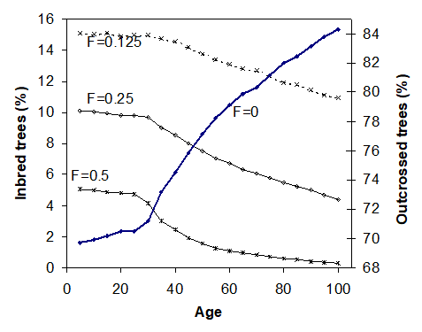
The TASS is a height-driven, biologically oriented, spatially explicit individual tree model (Mitchell 1975). It was designed to produce potential growth and yield tables for even-aged managed stands. It simulates the growth of individual trees in a three-dimensional space with competitions. Tree height, bole diameter, branch length, and crown form and foliage are updated annually. These measures can be affected by inter-tree competition, thinning, pruning, animal damage, site characteristics, defoliation, mortality, and fertilization, as well as genetic variation (or genetic treatments, as shown in Figure 6) in tree growth.

TASS can predict silvicultural treatment response by modelling individual tree crown dynamics and their relationship to bole growth and wood quality. This  makes TASS particularly well suited for predicting response to treatments such as

• Espacement,
• fertilization,
• pruning,
• pre-commercial and commercial thinning.

However, effects of climate change have not been incorporated into TASS models. Scientists are working on functions and parameters to link population response to climate into the modeling algorithms.

The software can be download for free at:

https://www2.gov.bc.ca/gov/content/industry/forestry/managing-our-forest-resources/forest-inventory/field-forms-and-software/software-download

4.4 LANDIS-II

The LANDIS-II forest landscape model simulates future forests (both trees and shrubs) at decadal to multi-century time scales and spatial scales spanning hundreds to millions of hectares. The model simulates change as a function of growth and succession and, optionally, as they are influenced by a range of disturbances (e.g., fire, wind, insects), forest management, land-use change. Climate and climate change affect processes throughout the model. LANDIS-II is highly customizable with dozens of libraries (‘extensions’) to choose from.

LANDIS-II is optimized for the simulation of spatial processes and the interactions between spatial processes and patterns. Landscapes within LANDIS-II are represented as a grid of interacting cells with a user-defined spatial resolution (cell size) and extent. Practicable cell sizes can range from a few meters up to a kilometer. All LANDIS models assume that individual cells have homogeneous light environments. Cells are aggregated into ecoregions with homogeneous climate and soils and a user-defined extent, thereby creating a hierarchy of spatial interactions.

The LANDIS-II community is very active with 100s of users and developers worldwide. Everyone is welcome to join the LANDIS-II community and to contribute. All model components are free and open-source. There are active bulletin boards for Users and Developers. And there are meetings and training held every year in various locations across the US and Canada.

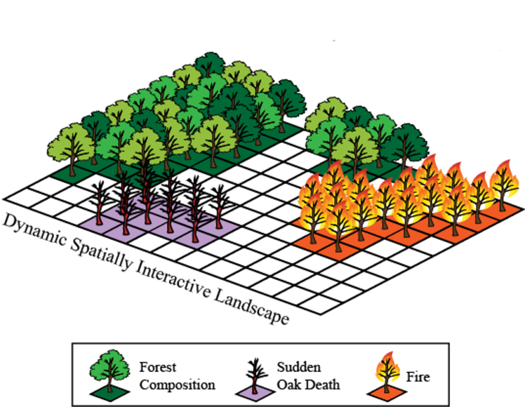
The following video shows an example of Landis II simulations:

The software of the model can be install from: http://www.landis-ii.org/install

By Tongli Wang, Climate Modelling and Forest Applications is licensed under Creative Commons <CC BY-NC-ND 4.0> License