Video #1 and #2: Concept of genecology

Video #3: Transfer functions:

Video #4: Genecology functions and predictors:

Contents

1. Overview
2. Definition of genecology
2.1. Definition
2.2. Some relevant terms
2.3. Objectives of genecology
3. Transfer functions
3.1. Provenance test
3.2. Transfer functions
3.3.  Features and limitations
4. General transfer functions
4.1.  General transfer functions
4.2. Relative performance-based general transfer functions
4.3.  Limitations of general transfer functions
4.4.  Universal transfer functions
5. Genecology functions
5.1. Genecology functions
5.2. The difference in genecology functions among environments
6. Geographic vs. climatic variables
6.1. Representation of environmental variables
6.2. Accessibility
6.3 local vs. universal
6.4. Applicability for climate change
6.5. Non-climatic factors

1. Overview

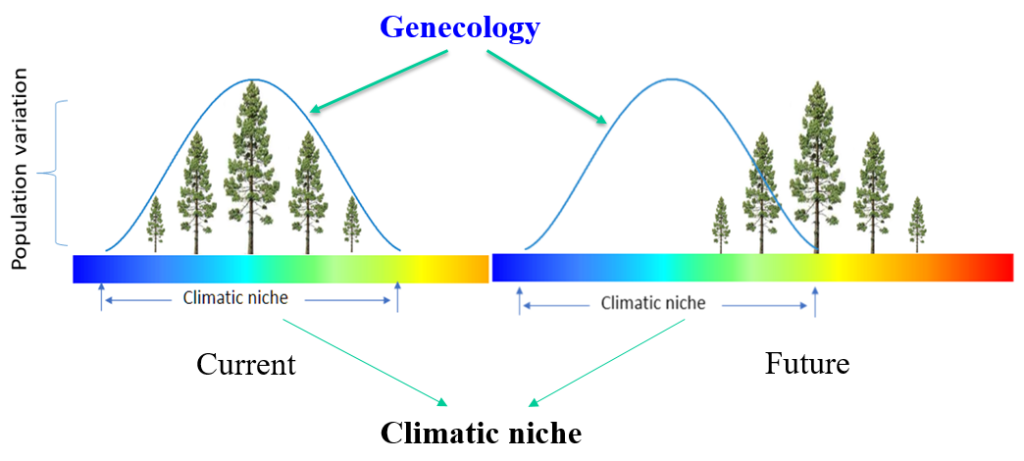
As mentioned in the previous topic and shown in Figure 1, climatic mismatches occur in two dimensions. One is the mismatch in the climatic niche at the species level (horizontally), and another is the mismatch at the population level (vertically). The niche-based models at the species level can be used to predict the shift in the climatic niche at the species level. Genecology functions are to predict among-population variations within a species.

2. Definition of genecology

2.1. Definition

Genecology is the study of intraspecific genetic variation in relation to environmental conditions. In other words, it is to study the relationships between genetic variation and environmental gradients within a species.

Genecology is often referred to as ecological genetics, which is actually more widely used. However, strictly speaking, ecological genetics is the study of how ecologically relevant traits evolve in natural populations, which covers inter-species interactions. Nevertheless, these two terms are used interchangeably.

2.2. Some relevant terms

Provenance – the place of seed origin (or seed source).

Population – a group of individuals of the same species that live in a particular geographical area, and have the capability of interbreeding. Individuals from the same provenance is called a population.

Provenance is often used to refer a population although it is not accurate. Thus, provenance and population are often interchangeably in genecology.

Provenance test (or provenance trial) – a common garden experiment that compares trees or plants collected from different provenances. Typically provenance tests compare widely separated seed sources. The test may contain multiple test sites.

Genetic variation – can be defined at the individual level as the difference in DNA among individuals, or at the population level as among-population variation due to difference in allele frequency.

Genetic cline – a geographic or climatic pattern of change in a trait.

Genetic and environment interaction (GxE) – different genotypes respond to environmental variation in different ways.

2.3. Objectives of genecology

Operational objectives:

• To determine how far seed can be moved
• To delineate geographic breeding zones
• To select optimal provenances

Theoretical objectives:

• Testing evolutionary and ecological theories about factors limiting the evolution of species range
• Predicting response to climate change
• Dependency on climatic drivers
• Determining the underlying genetic basis of adaptive traits: Ecological genomics

3. Transfer functions

Transfer functions are most commonly used in genecology to reflect the effect of transfer distance of populations in terms of geographical or climatic variables. A provenance test is required for developing a transfer function.

3.1. Provenance test

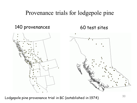
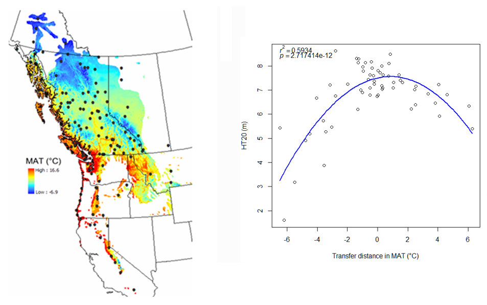
Figure 2 shows a typical provenance test. Populations from 140 provenances range-wide were planted in 60 common garden trials (planting sites) in British Columbia (BC), Canada. At each site, an incomplete block design was used to include 60 populations due to a large number of populations. Thus, not every population was tested at all the 60 sites except seven reference populations. Tree height was measured at age 20.

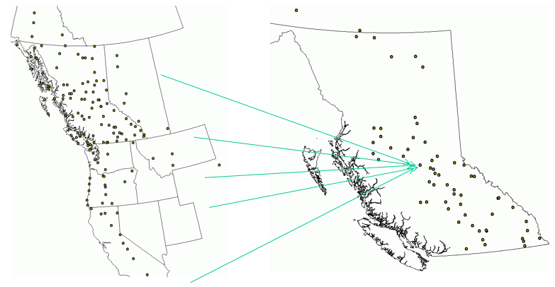
As illustrated in Figure 3, populations are transferred from their origins to a test site in the mid of BC in the provenance test. Those populations grow under new environmental conditions, and their performances may be affected. As the populations are grown under the same climatic conditions (at the same test site), the difference in the performance of populations is supposed to be due to genetic variation among the populations.

3.2. Transfer functions

The genetic variation observed in a provenance trial at each test site may be associated with the population transfer distance. It is hypothesized that the longer the transfer distance, the larger the transfer effect. Thus, the transfer distance is used as a predictor in a transfer function as:

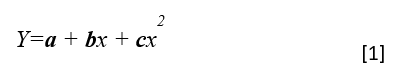
Where, Y is the performance of a population; x is the transfer distance; and a, b, and c are parameters to be estimated to fit the model.

The transfer distance can be in a physical distance for geographical variables (e.g., latitude, longitude, or elevation), or in units for climatic variables (e.g., temperature and precipitation). Climatic variables are increasingly used as they have many advantages over geographical variables, particularly for predicting the impact of climate change on forests.

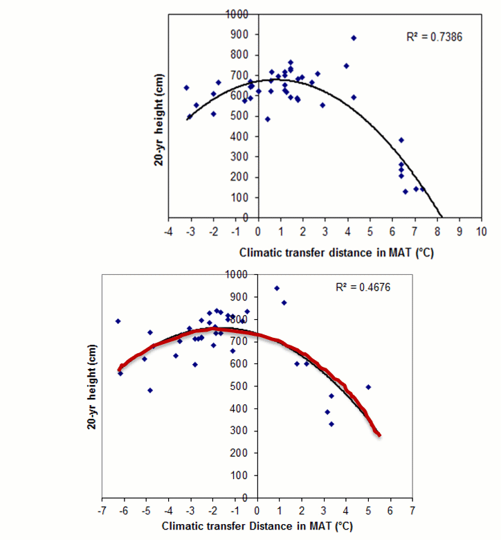
Climatic variables are needed for all the provenances to build a transfer function using the transfer distance in climatic variables, as shown in Figure 4. A map of mean annual temperature (MAT) covering the lodgepole pine distribution and a transfer function for a test in the mid of BC.

The transfer distance in MAT (MAT_CTD) is calculated as:

MAT_CTD = MAT_s – MAT_p                         [2]

Where, MAT_s is the MAT of the test site, MAT_p is the MAT of the provenance. Then, the transfer function is written as:

Populations with negative transfer distances on the left of the plot were transferred northward (from warmer climates to cooler climates). On the other hand, populations with positive transfer distances on the right of the plot were transferred southward (from cooler climates to warmer climates).  Populations with zero and around zero transfer distance are considered local populations. The local populations have the best performance; however, the peak of the curve is not always exactly at the zero transfer distance point, as shown in Figure 4.

3.3.  Features and limitations

A transfer function represents the transfer effect of populations. It reflects the genetic effect of climate on populations. It is intuitive and easy to build. However, there are several limitations for transfer functions. A transfer function built for one site may be different from the one built for another site, even with the same group of populations. Thus, a transfer function developed for one site, strictly speaking, only represents the transfer effect of populations under the particular environment of that test site. The number of test sites is limited for most tree species, and people tend to oversell the results drawn from these sites. Therefore, we need to be aware of such a risk of using a transfer function built for one environment to represent the situations for other environments.

4. General transfer functions

4.1.  General transfer functions

Due to the limitation of transfer functions discussed above, general transfer functions were proposed. The only difference between a transfer function and a general transfer function is that data from all test sites are pooled together in developing a general transfer function. The formulas [1] – [3] all apply to a general transfer function.

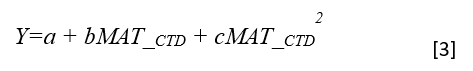
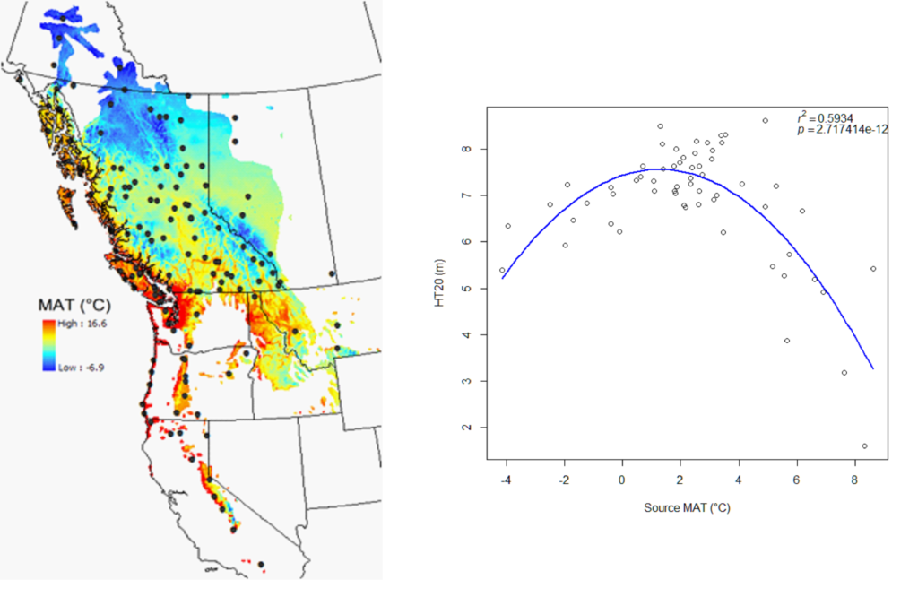
The curve of a general transfer function shown in Figure 5 was developed based on the observations from the same provenance test mentioned above. The relationship between the performance and transfer distance of populations in a transfer function is usually weak.

4.2. Relative performance-based general transfer functions

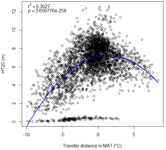
The most important reason for a general transfer function being weak is the difference in the performance of populations among sites. For example, the outliers at the bottom of Figure 5 are populations growing at several cold sites in the north. Their total height at age 20 is less than a meter. An approach was developed to overcome this problem by using relative performance. With this approach, the performances of populations are converted to proportions relative to the performance of the local population.  It can substantially improve the relationship of the general transfer function, as shown in Figure 6. It worths of reminding that the relative performance needs to be converted back to actual performance in applications of this model.

4.3.  Limitations of general transfer functions

In addition to the weak relationships of general transfer functions as mentioned above, there are other limitations for general transfer functions. As discussed earlier, the transfer effects of populations are different among test sites. By pooling the data across all test sites to develop a general transfer function, the difference in the transfer effect of populations among test sites is averaged out, as illustrated in Figure 7. This compromises the prediction power of general transfer functions. In addition, the same amount of transfer distance may have different transfer effects. For example, for a -2°C transfer distance in temperature, the transfer from 2°C to 0°C may be different from the transfer from 10°C to 8°C. This point will be further discussed later in comparison with genecology functions. Nevertheless, general transfer functions are the simplest to implement; thus it is still commonly used.

4.4. Universal transfer functions

Where,
X is transfer distance;
P is provenance climate;
XP is the interaction term;
rs are some random effect terms.

The universal transfer function can overcome the problems listed above, but the random terms cause additional problems. The model is too complicated and often fail to converge. It used only one climate variable in applications so far, which can compromise the model capability.

.

5. Genecology functions

5.1. Genecology functions

A genecology function uses the environmental variables of provenances, rather than transfer distance used in both transfer functions and general transfer functions. Thus, a genecology function represents the relationship between the performance of populations and environmental variables of the population origins (or provenances), which exactly reflects the definition of genecology. A genecology function can be written as:
Y=a + bx + cx²
Where, Y is the performance of a population; x is an environmental variable of provenance; and a, b, and c are parameters to be estimated to fit the model.

Using the same data for building a transfer function in Figure 4, a genecology function is developed, as shown in Figure 8. Although the shapes of the curves are quite different, the R square values are identical between the two functions.

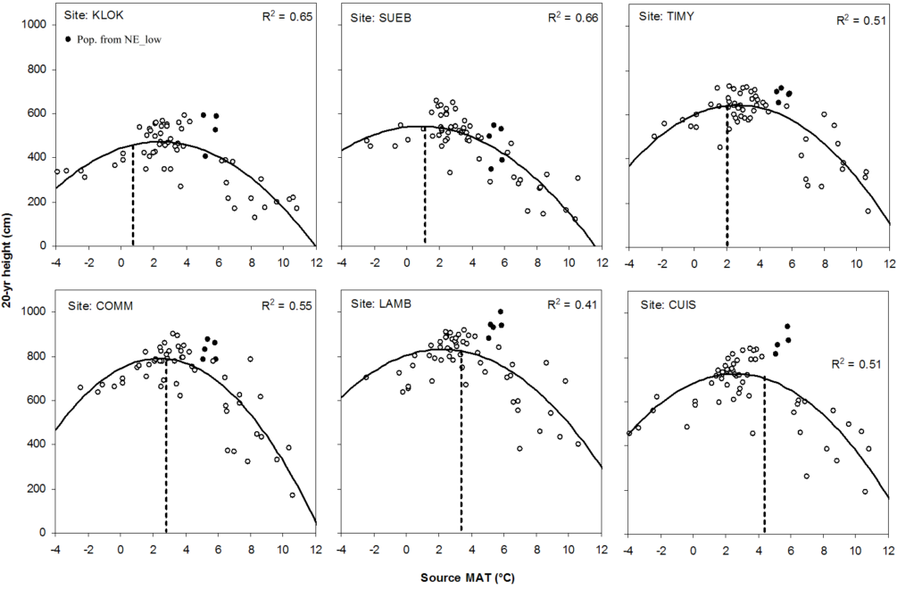
5.2. The difference in genecology functions among environments

Genecology functions developed for different environments show different relationships (Figure 9). Thus, a genecology function built based on information from one environment may not represent the relationship for other environments. This is the same as for the transfer function.

6. Geographic vs. climatic variables

Both transfer functions and genecology functions can be built with either geographic or climatic variables. There are advantages and disadvantages to use geographic or climatic variables as predictors. We will make a detailed comparison between the two.

6.1. Representation of environmental variables

Geographic variables are not direct environmental variables, whereas climatic variables are. However, geographic variables are related to environmental variables. For example, elevation is strongly related to temperature, which affects plant performance, as illustrated in Figure 10. Thus, they are often used to substitute environmental variables. However, if we build a greenhouse at the top of the mountain, we can grow any plant that can only grow at the bottom of the valley. It suggests elevation itself does not affect plant growth.

6.2. Accessibility

Geographic variables are more accessible than climatic variables. That is why they were more often used for experimental design and data analysis in the past. With increasingly available climate data, accessing climatic variables are becoming as easy as accessing geographic variables. Especially with the scale-free climate models ClimateNA and ClimateAP, climatic variables can be easily obtained for any specific location within their coverage.

6.3 local vs. universal

A transfer function or a genecology function built with geographic variables only works for the region where the model is built. This is because of the effect of a geographic variable changes from region to region, or location to location. For example, 2000 m in elevation in California is suitable for many plants to growth; but the same elevation in BC is beyond the treeline. Also, an increase in elevation by 100 m in California will result in a decrease in temperature by 0.65°C; but the same change in northern BC will only result in a decrease in temperature by about 0.2°C.  In contrast,  a transfer function or a genecology function built with climatic variables can be applied anywhere.

6.4. Applicability for climate change

A transfer function or a genecology function built with geographic variables cannot be used for assessing the impact of climate change as geographic variables are static and have no future projections. In contrast, climatic variable based functions can predict the past and future. That is the reason why genecology has been a hot area.

6.5. Non-climatic factors

Geographic variables are still useful to reflect some important non-climatic factors. Genetic variations among populations are also affected by spatial autocorrelation involving migration and gene flow related to physical barriers and distance. Those factors sometimes need to be included in genecology functions. We will discuss this further in the next topic.

By Tongli Wang, Climate Modelling and Forest Applications is licensed under Creative Commons <CC BY-NC-ND 4.0> License