4 Topic 3.2. Using ClimateNA/AP to Generate Point and Spatial Climate Data
Note: Tutorial videos are embedded within the related content below. Thus, no additional videos are provided here.
Contents
1. Download and installation
1.1. Download
1.2. Installation
2. Using the interactive mode
2.1. Coordinates input
2.2. Period selection
2.3. Climate data generating and saving
3. Using multi-location mode
3.1. Input file preparation
3.2. Multi-location processing
4. Multiple GCMs and RCPs processing
5. Generating spatial climate data
5.1. Installing R packages
5.2. Preparing an input file from a DEM file
5.3. Using a DEM as an input file
6. Using time-series functions
6.1. Historical Time Series
6.2. Future time series
6.3. Time-series raster files
7. Using the web version
7.1. Easy access to climate data
7.2. Visualizing spatial climate variables
7.3. Visualizing ecological niche maps of tree species and forest ecotypes
8. Using pre-generated spatial data
1. Download and installation
1.1. Download
ClimateNA and ClimateAP are free for download from their websites at
http://climatena.ca/ and http://web.climateap.net/
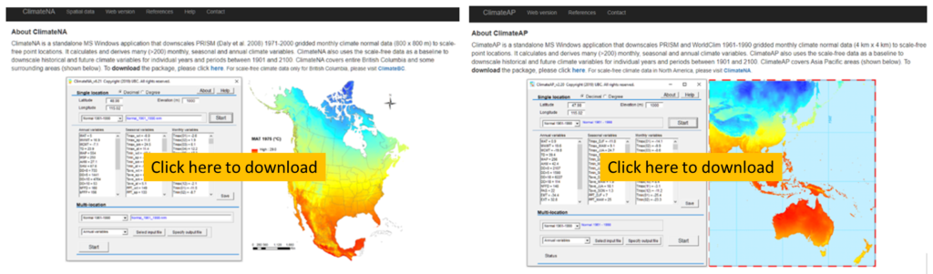
By clicking on the interface of each model, you will be led to the downloading page. To download, users are required to register to a mailing list first, which is only for informing new releases and important announcements. After the registration, a downloading link will appear on the page and also be sent to your email. The packages are compressed zip files with sizes of about 600 MB for ClimateNA and 300 MB for ClimateAP.
1.2. Installation
No installation is required. Users just need to simply unzip all the files and subfolders into a folder on your hard disk and double-click the file ClimateNA _v6.**.exe”. The program does not work on network drives for some unknown reasons.
The exe file can be started even without uncompress the package. However, it does not work properly, and an error message will appear if the “Start” button is clicked.
The program runs on all Windows. It can also run on Linux, Unix and Mac systems with the free software Wine or MacPorts/Wine.
A Youtube video is available to demonstrate the steps of downloading and installation.
Video 1. A tutorial for downloading and installation of ClimateNA (or ClimateAP). Video by Tongli Wang under CC BY 4.0.
2. Using the interactive mode
2.1. Coordinates input
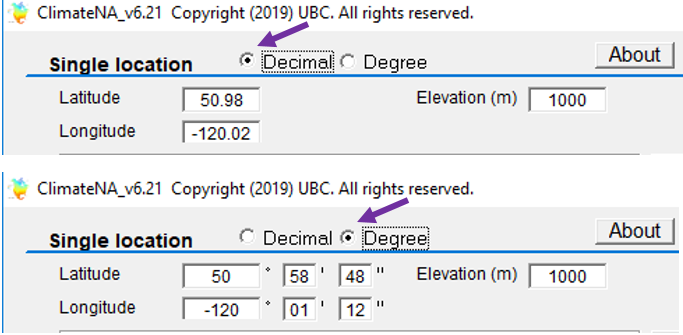
The upper section of the interface is for processing single locations. Users need to manually type in the latitude, longitude, and elevation of a location of interest.
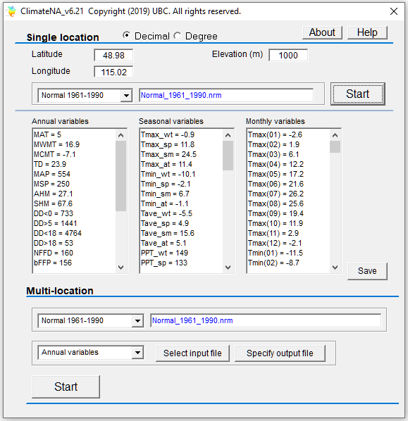
The latitude and longitude can be in decimal degrees with the default option. They can also be in degree, minute and second if the “Degree” option is selected. Elevatopm is always in meters. If elevation is missing (or not available), the program still generates climate data based on the bilinearly interpolated elevation values of the baseline dataset, thus, elevation adjustment is not applied in that case.
2.2. Period selection
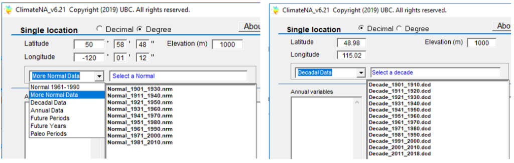
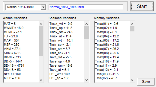
The default period in both ClimateNA and ClimateAP is the normal period 1961-1990, which is also the period defined as a standard reference period for long-term climate change assessments by the World Meteorological Organization.
More normal period – selection for more normal periods is available by selecting “More Normal Data”. There are nine normal periods available over the period of 1901-2019.
Decadal data – a decadal period can be selected in the same as for selecting a normal period. There are 12 decadal periods available including an incomplete decadal period for the current decade (2011-2018).
Annual data – to generate climate data for a specific year, “Annual Data” needs to be selected in the period dropdown menu. A list of all years will appear for the period of 1901-2019, and an individual year can then be selected.
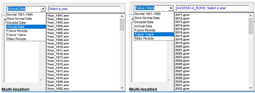
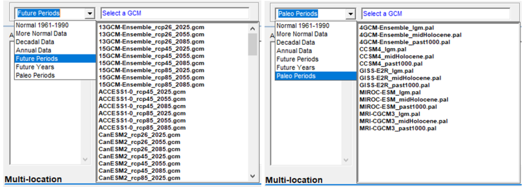
Future periods – A General Circulation Model (GCM), a Representative Concentration Pathway (RCP), and a future period can be selected under “Future Periods”. There are 15 GCMs for the greenhouse gas emission scenarios RCP4.5 and RCP8.5, and 13 GCMs for RCP2.6. There is also ensemble for each RCP and period over all the GCMs. These ensembles are widely used in climatic and ecological modelling applications.
2.3. Climate data generating and saving
After a period is selected as mentioned above, it is ready to generate climate data by clicking on the “Start” button. Data generated for annual, seasonal and monthly climate variables are shown in Figure 7. The data values and the coordinates and elevation can be saved as a CSV file by clicking the Save button.
3. Using multi-location mode
The lower section of the interface of the programs is for processing multiple locations. It requires users to prepare an input file that comprises identifications, latitude, longitude and elevation of the locations of interest. The output file keeps all the columns of the input file, but attach climate variables to each location (or each row). Since version 6.0, ClimateNA can also directly read a digital elevation model (DEM) and generate output files in raster format for mapping. The multi-location mode allows time-series functions to generate climate data for multiple years and processing multiple GCMs, RCPs and periods in a single run.
3.1. Input file preparation
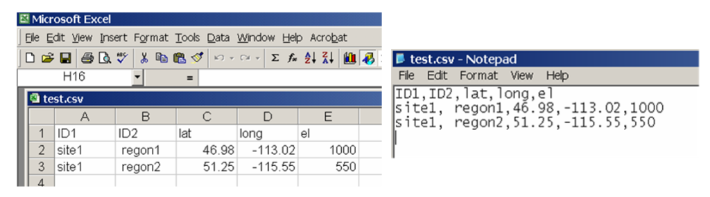
An input file can be prepared either in Microsoft Excel, a text editor or R. The file must comprise five columns with the first two columns for IDs (e.g., “ID” and “Site” ) and three columns for latitude (lat), longitude (long), elevation (el) as shown in the example below. The columns must be in the same order as shown. If elevation is not available, you have to put in “.” Instead and no elevation adjustment will be applied to that location. No additional columns are allowed. The input file can have almost unlimited number of locations (or rows).
If the file is prepared in Excel, it must be save as a comma-delimited spreadsheet file (a CSV file). If the file is prepared in a text editor, the values must be separated by comma (“,”). If there is a missing value, you need to enter a “.” between two commas. If prepared in R, it need to be save using “write.csv” command.
For making climate maps, an input file can also be converted from a digital elevation model (DEM). This will be explained later in this lecture.
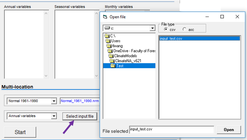
3.2. Multi-location processing
After selecting a period and climate variables, you can select your input file, for example, “Input_test.csv”. Then, click the “Open” button.
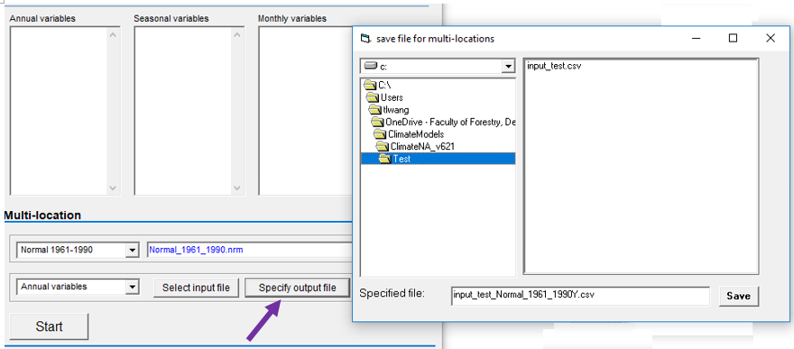
The next step is to specify an output file by clicking on the “Specify output file” button. A default output file name is provided, which contains all the information about the input file, period and climate variable category. You may not need to change it in most cases. Then, it is ready to hit the “Start” button to run the process.
A Youtube tutorial shows all the steps and more.
4. Multiple GCMs and RCPs processing
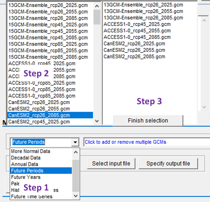
In multi-location mode, climate data can be generated for multiple GCMs, RCPs and periods in a single run. Here are the steps:
- 1) Click on “Future Periods” in period selection dropdown box, and a list of GCMs, RCPs and periods will appear on the left.
- 2) Click on the items in the list to make selections, and selected items will appear in the list on the right. If an item is selected by mistake, it can be removed from the list by clicking on it.
- 3) After the selection is completed, click on the “Finish Selection” button.
- 4) Select climate a variable category, open an input file and specify an output file name.
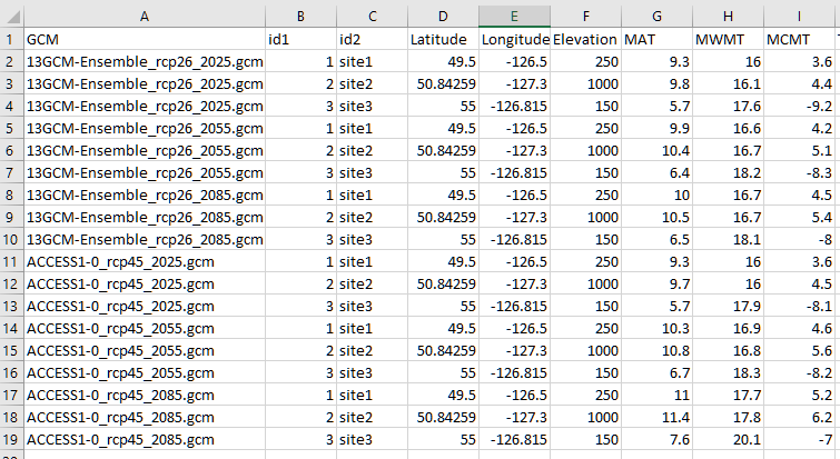
All the climate data are generated in one output file. A column is added on the left to show the information of the GCM, RCP and period.
All the steps are also shown in a Youtube:
5. Generating spatial climate data
ClimateNA and ClimateAP can generate spatial climate data at any spatial resolution. A DEM file is required either for preparation of an input file for ClimateAP or directly used as an input file for ClimateNA. The spatial resolution of the DEM file determines the spatial resolution of the output raster files.
5.1. Installing R packages
We need R to prepare input files and to process output data. Here we will show the steps to install R on Windows, and to install and load R packages. As we will provide the code for each processing work, no programming is required for this lecture. Here are the steps:
1) Download R: https://cran.r-project.org/bin/windows/base/R-4.0.3-win.exe
2) Click to run the exe file “R-4.0.3-win.exe. Follow the instruction on the screen to complete the installation.
3) Click the newly installed R-4.0.3 to start R.
4) Click “File”, then “New script” to open the R code editor
5) Type “install.packages(‘raster’)” and run it by right click and select “Run line or selection”, and follow the instruction on the screen to complete the package installation.
Now you are ready to run the code provided later on.
5.2. Preparing an input file from a DEM file
DEM files can be obtained from various sources. For example, free Digital Elevation Models can be downloaded at https://www.opendem.info/link_dem.html. However, to get a DEM for a specific area is not readily available. The following Youtube tutorial video shows you how.
A simple way to convert a DEM file into an input file for ClimateAP is to do it in R. The following code is used to convert the DEM file “bc80k.asc” in ascii raster format (or “bc80k.tif” in tiff format) to an input file in CSV format (“bc80k.csv”) using raster package (R package can be downloaded at https://www.r-project.org/):
library(raster);
setwd(‘ your working folder‘)
r <- raster(‘bc80k.asc’);
xye <- rasterToPoints(r);
yxe <- cbind(lat=xye[,2],lon=xye[,1],elev=xye[,3]);
yxe2 <- data.frame(ID1=row(xyv)[,1],ID2=row(xyv)[,1],yxe);
write.csv(yxe2,’bc80k.csv’,row.names=F)
A DEM file can be converted into an input file either in ArcGIS Map, Python or other programs as long as the output file meets the requirements as mentioned in 3.1.
ClimateAP or ClimateNA can use this input file to climate data in CSV format as shown in 3.2. To convert the CSV file (e.g., “bc80k_1975Y.csv”) into spatial layers, the following code can be used in R for MAT as an example:
library(raster);
setwd(‘ your working folder‘)
csv <- read.csv(‘bc80k_1975Y.csv’);
MAT <- rasterFromXYZ(csv[,c(4,3,6)]);
plot(MAT)
5.3. Using a DEM as an input file
Since version 6.0, ClimateNA can directly read a DEM raster file as an input file and generate climate variables in raster format for mapping. This makes it much easier to generate spatial climate variables. Here are the steps:
- Have a DEM raster file (*.asc) for the area of interest at the resolution you want;
- Click the “Select input file” button and a file open box will show up;
- Navigate to the folder containing the raster file;
- Select the File type: “asc” as shown in the following screenshot and only asc raster files will show up:
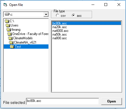
Figure 13. A screenshot of the file-open box to illustrate the selection of a raster input file. Image by Tongli Wang under CC BY 4.0. - Select an asc input file and click “Open” button;
- Click the “Specify output file” button, and a default folder will show up
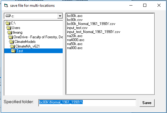
Figure 14. A screenshot of file-save box for specifying an output folder. Image by Tongli Wang under CC BY 4.0. - Click the “Save” button;
- Click the “Start” button, and climate variables in ASCII raster format will be generated;
- Projection: geographic coordinate system, GCS_WGS_1984.
- Data format: the following variables were multiplied by 10:
- Annual: MAT, MWMT, MCMT, TD, AHM, SHM, EMT, EXT and MAR;
- Seasonal: Tmax, Tmin, Tave and Rad;
- Monthly: Tmax, Tmin, Tave and Rad.
- Drag and drop an output file into ArcGIS to show the map, or display the map in R using the following code:
library(raster);
setwd(‘ your working folder‘)
mat <- raster(‘mat.asc’);
plot(mat)
A Youtube video shows the steps:
6. Using time-series functions
ClimateNA and ClimateAP can generate time-series climate data for historical (1901-2018) or future years (2011-2100) for multiple locations in a single run. The time-series functions work only for the multi-location process.
6.1. Historical Time Series
Here are the steps to generate historical time-series climate data:
- 1) Select “Historical Time Series” in the period selection dropdown box;
- 2) Select a variable category (monthly, seasonal, annual or all variables);
- 3) Input the starting and ending years in the pop-up boxes;
- 4) Specify input and output files, and click the “Calculate TS” button.
The climate data for all the years involved will be saved in a single CSV file. The information of years is added as the first column to the output file. The size of the file can be huge.
6.2. Future time series
The steps are slightly different for generating time-series data for a future period as it involves selection of GCM, RCP and GCM model runs. Here are the steps:
- 1) Select “Future Time Series” in the period selection dropdown box;
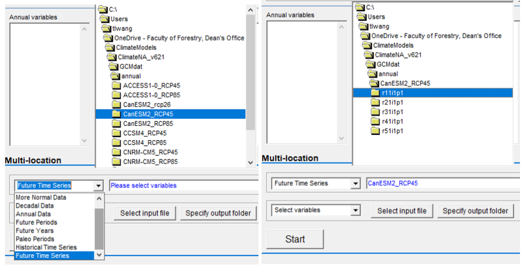
- 2) Select a variable category (monthly, seasonal, annual or all variables);
- 3) Input the starting and ending years in the pop-up boxes;
- 4) Specify input and output files, and click the “Calculate TS” button.
6.3. Time-series raster files
The two time-series functions also work for generating spatial raster files. The only differences in the steps include:
- 1) Select an ASCII raster input file as in 5.2;
- 2) Specify an output folder instead of an output file. Although the default folder works in most cases, this step cannot be skipped.
The following Youtube video shows all the steps mentioned above.
7. Using the web version
The web versions of ClimateNA and ClimateAP can be accessed at: http://www.climatewna.com/default.aspx
http://climateap.net/default.aspx
7.1. Easy access to climate data
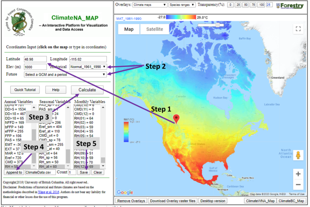
Different from the desktop versions, typing in coordinates is optional as they can be automatically obtained by clicking on the Google Map. There are two dropdown boxes for selecting either a historical period or years, or a future period. There are only three GCMs available in contrast to 15 GCMs in the desktop versions. Here are the steps:
- 1) Click at the location of interest on the Google Map and the lat, lon and elve will be automatically obtained through Google Service. Alternatively, lat, lon and elve can be typed in.
- 2) Select either a historical or a future period;
- 3) Click the “Calculate” button to generate climate data;
- 4) Click the “Append” button to save the climate data to the temperate memory;
Get climate data for other locations or periods by repeating the steps 1) – 4);
- 5) Click the “Save” button to save the data to your local computer.
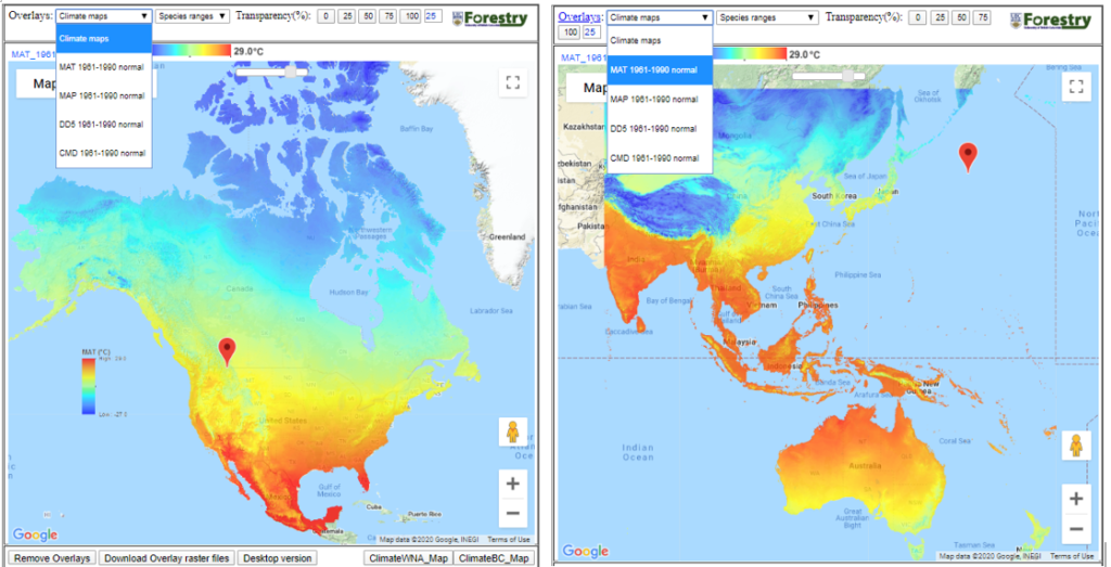
7.2. Visualizing spatial climate variables
Several major climate variables are overlaid on the Google Maps and they can be visualized using the Google Map features. When a climate variable is shown, it can be downloaded as a raster file to your local computer by clicking on “Download overlay raster files”.
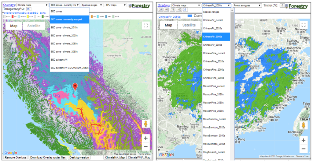
7.3. Visualizing ecological niche maps of tree species and forest ecotypes
Ecological niche maps of some major forest tree species are also overlaid onto the Google Maps in ClimateNA and ClimateAP, and their subprograms, such as ClimateBC_Map and ClimateChina.
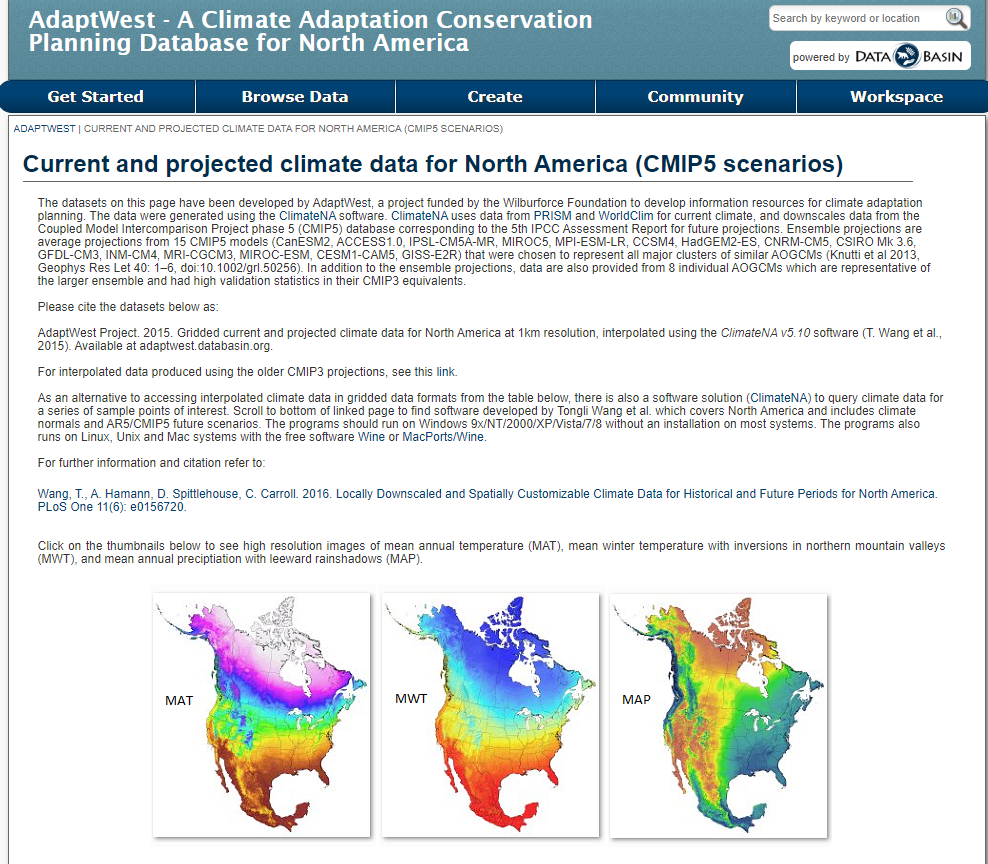
8. Using pre-generated spatial data
A large volume of pre-generated spatial climate data using ClimateNA is available for download. However, such spatial data are not available yet for ClimateAP.
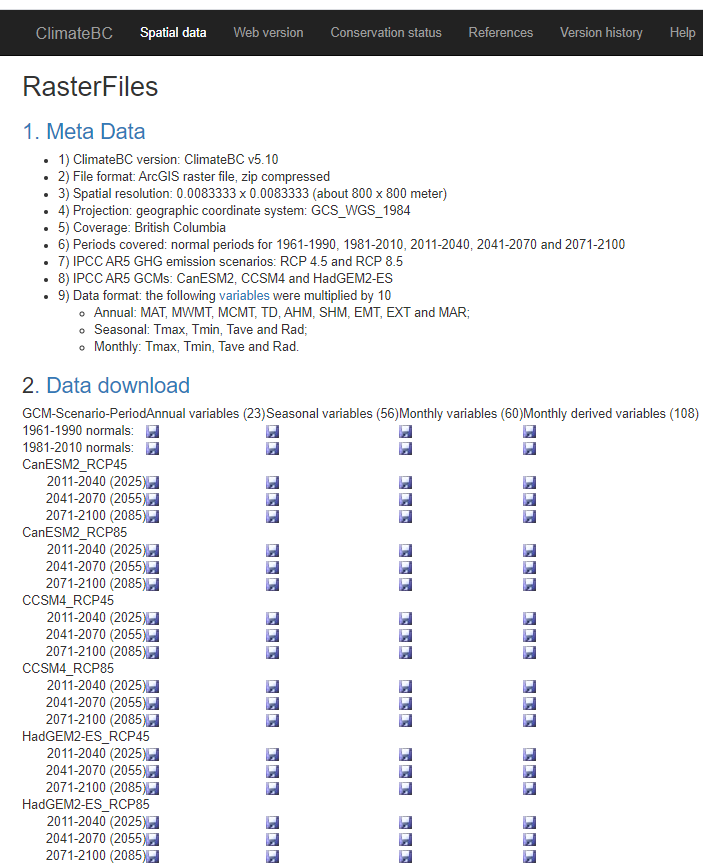
Figure 19. Pre-generated spatial climate data in ClimateBC. Image by Tongli Wang under CC BY 4.0.
Steps to download such spatial data are provided at the websites and straightforward. Our next step is to develop an application programming interface (API) based database for spatial climate variables.

By Tongli Wang, Climate Modelling and Forest Applications is licensed under Creative Commons <CC BY-NC-ND 4.0> License
