Video #1: Introduction to ClimateNA and ClimateAP – Overview:

Video #2: Introduction to ClimateNA and ClimateAP – How do they work?

Video #3: Introduction to ClimateNA and ClimateAP – Main features:

Contents

1. Overview
2. Data sources
2.1. Baseline data
2.2. Historical data
2.3. Future climate data
2.4. Paleoclimate data
3. Dynamic local downscaling
3.1. Baseline data
3.2. Historical and Future climate data
4. Development of additional climate variables
4.1. Calculated climate variables
4.2. Derived climate variables
5. Main features
5.1. Scale-free climate data
5.2. All-in-one package
5.3. Multiple-location and multiple-GCM processing
5.4. Time-series functions
5.5. Map-in and map-out capacity
6. Web versions
7. Spatial data

1. Overview

ClimateNA and ClimateAP are standalone MS Windows software packages that generate scale-free climate data for historical (1901 – 2019), future (2011-2100) and paleo (back to 21,000 years back) periods and years. They also calculate and derive many (>200) monthly, seasonal and annual climate variables to facilitate ecological modeling.  Time-series functions are available to generate climate variables for multiple locations and multiple years for historical or future years in a single run.

The scale-free feature allows users to generate climate data for specific locations (instead of grid averages from other climate models) for better accuracy and to generate climate surfaces at any spatial resolution, which is particularly useful for applications at regional and local scales. The scale-free feature is achieved through a dynamic local downscaling to the gridded climate data from PRISM and WorldClim.

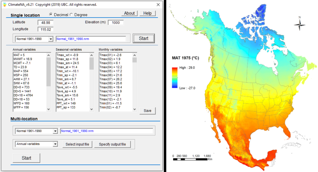
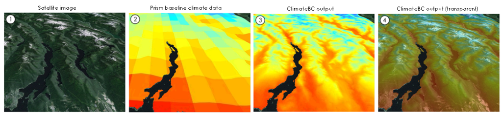
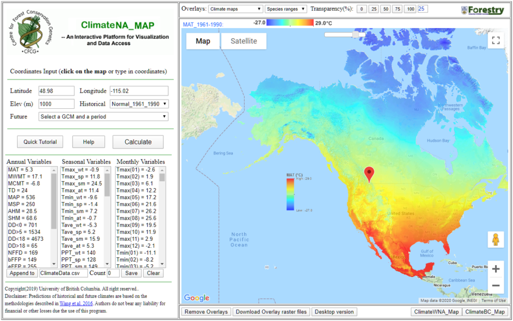
The application packages can be downloaded for free. No installation is required. The program can read and output comma-delimitated spreadsheet (CSV) files. The new version of ClimateNA (v6.00) can also directly read digital elevation model (DEM) raster (ASC) files and output climate variables in raster format for mapping. The spatial resolution of the raster files is up to the user’s preference. ClimateNA covers the entire North America (Figures 1).

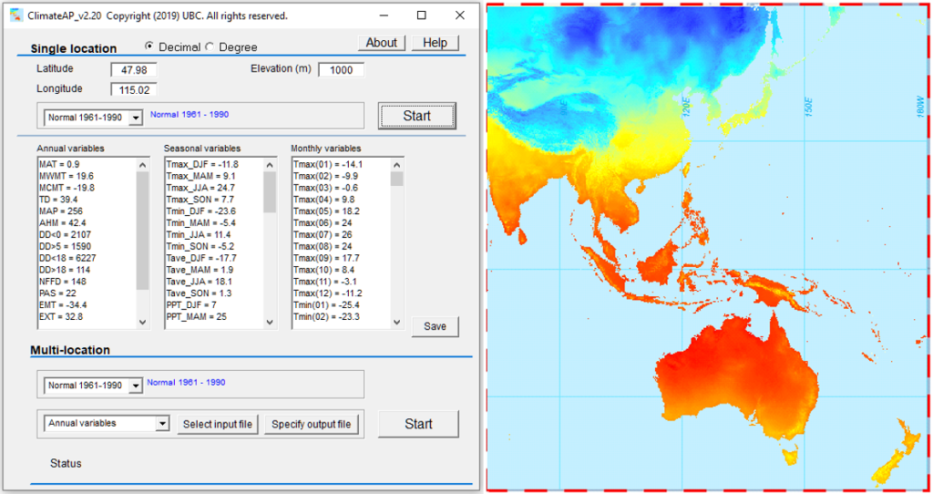
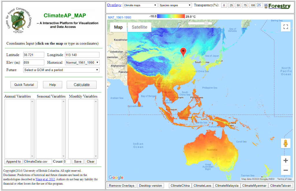
ClimateAP covers a major part of the Asia Pacific region (Figure 2).

ClimateNA and ClimateAP have been widely in climate change-related studies and applications in almost all fields including forestry, forest genecology, plant ecology, hydrology, meteorology, and agriculture. Currently, there are over 1,500 subscribers and a total of over 1,600 citations.

2. Data sources

2.1. Baseline data

The monthly baseline data for 1961-1990 normals were compiled from the following sources and unified at 4 x 4 km spatial resolution:

• British Columbia: PRISM at 800 x 800 m from Pacific Climate Impact Consortium;
• Parries provinces: PRISM at 4 x 4 km from the PRISM Climate Group (http://www.prism.oregonstate.edu/);
• United States: PRISM at 800 x 800 m from the PRISM Climate Group (Daly et al. 2008);
• The rest: WorldClim (Hijmans et al. 2005);
• The monthly solar radiation data (1948-2010) were provided by Dr. Robbie Hember at the University of British Columbia (to be replaced soon).

2.2. Historical data

Historical monthly data are developed by ourselves for ClimateNA. For ClimateAP, the historical monthly data are from the Climate Research Unit (CRU ts4.04). Both datasets are provided at the spatial resolution is 0.5 x 0.5° and updated annually.

2.3. Future climate data

The climate data for future periods, including the 2020s (2011-2040), 2050s (2041-70), and 2080s (2071-2100), were from General Circulation Models (GCMs) of the Coupled Model Intercomparison Project (CMIP5) included in the IPCC Fifth Assessment Report (IPCC 2014). Fifteen GCMs were selected for three greenhouse gas emission scenarios (RCP2.6, RCP4.5 and RCP8.5) except two GCMs that do not have data for RCP2.6. When multiple ensembles are available for each GCM, an average was taken over the available (up to five) ensembles. Ensembles among the 15 GCMs are also available. Time-series of monthly projections are provided for the years between 2011-2100 for RCP4.5 and RCP8.5 of six GCMs.

2.4. Paleoclimate data

ClimateNA (not yet in ClimateAP) contains monthly paleoclimate data were from four GCMs of the CMIP5. The paleo periods covered: 1) Last Millennium or past 1000 years, starting on January 01, 0850; 2) MidHolocene (6,000 years ago); and 3) Last Glacial Maximum (21,000 kyrs ago). Monthly averages were taken over the first 50 years of each period, which is the minimum period available in among the four GCMs.

3. Dynamic local downscaling

3.1. Baseline data

Instead of using the midpoint values of each grid cell to represent all locations in the grid, ClimateNA and ClimateAP use a combination of bilinear interpolation and local elevation adjustment approaches to downscale the baseline monthly grid data (4 × 4 km) to scale-free point locations. In other words, the programs predict climate data for every specific location.

The program first uses bilinear interpolation to estimate values between midpoints of the four neighbor grids to generate a seamless surface for each monthly climate variables, avoiding step-artifacts at grid boundaries.

The algorithms then retrieve monthly climate data and elevation values for a location from the corresponding grid cell plus eight surrounding cells. The climate and elevation values of the nine cells are used to calculate differences in a climate variable and in elevation between all 36 possible pairs. A simple linear regression of the differences in the climate variable on the difference in elevation is then established, and the slope of the regression is used as the empirical lapse rate for each climate variable at each specific location. The lapse rates are estimated for all the 48 primary monthly variables in ClimateNA and 36 in ClimateAP.

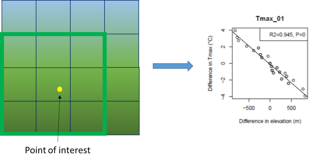
To avoid over-adjustments due to a weak linear relationship, each lapse rate was weighted by the R-square value of the local linear regression. The estimated lapse rate is applied to adjust the bilinearly interpolated values of the location to achieve the downscaling. As the local regressions are dynamically developed along with locations of inquiry, this downscaling method is called a “dynamic local downscaling” approach.

3.2. Historical and Future climate data

Historical, paleo, and future climate data are first converted to anomalies relative to the reference normal period (1961-1990), bilinearly interpolated, then added onto the downscaled baseline monthly climate normal data (scale-free) to arrive at the final climate surface at a specified resolution or for point data. This approach is called a delta downscaling approach, as illustrated in Figure 5.

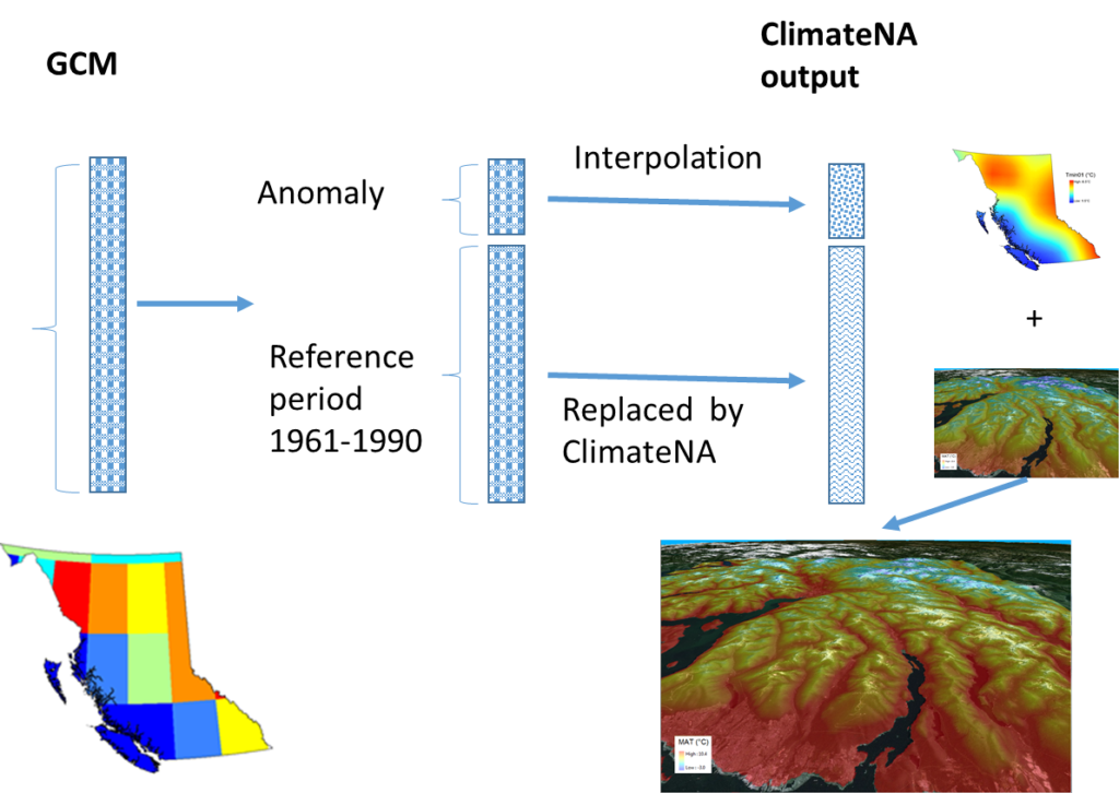
With this approach, the original baseline portion (i.e., absolute values for the 1961–1990 normal period) of the historical and future climate data were replaced by the scale-free climate data generated by ClimateNA. Because elevation-adjusted baseline data generated by ClimateNA typically has much higher spatial resolution and accuracy than the historical and future climate data, this process improved the accuracies for both historical and future climate data. However, the approach does not change or improve the anomaly portions of the historical and future climate data except the effect of bilinear interpolation.

4. Development of additional climate variables

The baseline dataset contains 36 primary monthly climate variables, including monthly minimum (Tmin) and maximum (Tmax) temperatures, and monthly total precipitation (Prep). ClimateNA and ClimateAP generate over 200 biologically relevant climate variables to facilitate applications in ecology and forest resource management. Of these climate variables, some are directly calculated from the primary monthly climate variables, and others are derived (or estimated) based on observations from weather stations.

4.1. Calculated climate variables

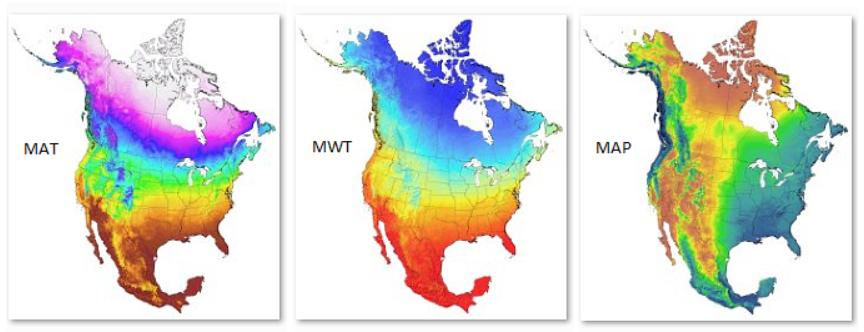
Monthly mean temperatures (Tave) are calculated from monthly Tmin and Tmax. Annual and seasonal mean temperatures and total precipitation are calculated from Tave and Prep, such as mean annual temperature (MAT) and mean annual precipitation (MAP). Other often-used annual climate variables include mean warmest month temperature (MWMT), mean coldest month temperature (MCMT), continentality (TD), which is the difference between MWMT and MCMT, and mean summer precipitation (MSP), ect.. A full list of calculated climate variables can be found at http://climatena.ca/

4.2. Derived climate variables

Many of these additional variables need to be calculated using daily climate data, which are not available in ClimateNA. We estimated these variables based on empirical or mechanistic relationships between these variables calculated using daily observations and monthly climate variables from weather stations from entire North America for ClimateNA, and from the Asia Pacific for ClimateAP. We called these variables “derived climate variables”. These variables were developed at the monthly scale, then summed up to seasonal and annual scales. The steps included: 1) calculating derived climate variables for each month (e.g., degree days) from daily weather station data; 2) building relationships (or functions) between the derived climate variables and observed (or calculated) monthly climate variables; 3) applying the functions in ClimateNA and ClimateAP to estimate derived climate variables using monthly climate variables.

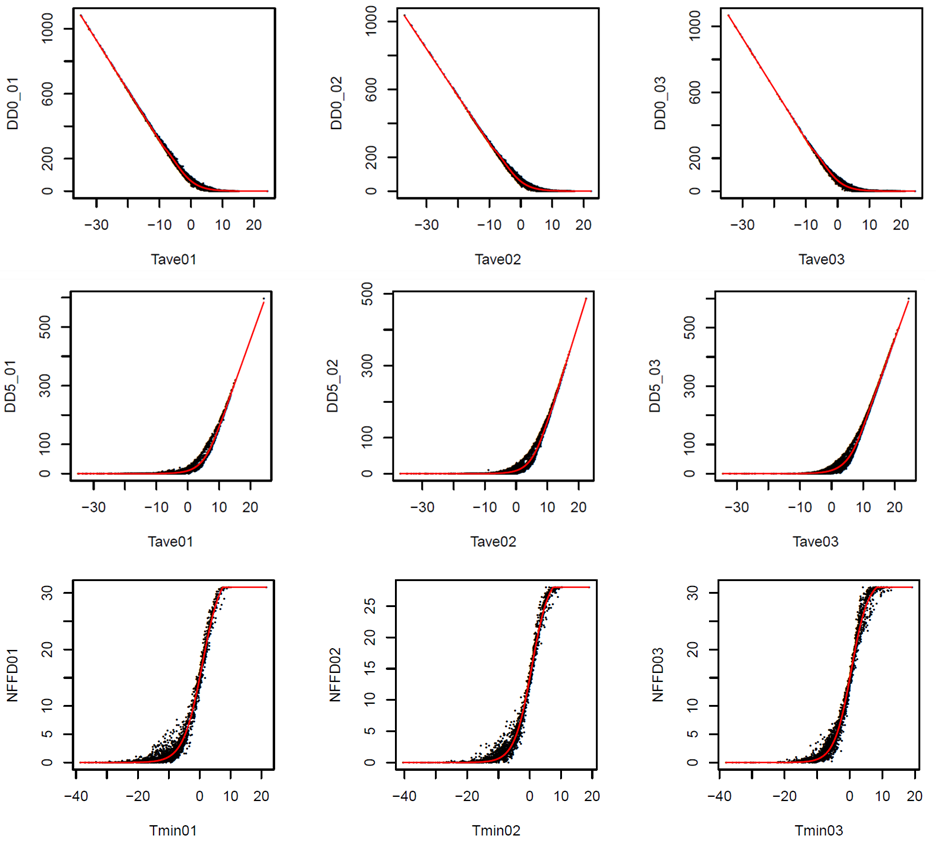
The widely used derived climate variables include growing degree-days (DD>5), cooling degree-days (DD<0), frost-free days (NFFD), frost-free period (FFD), extreme minimum (EMT) and maximum (EXT) temperatures, and climatic moisture deficit (CMD). A full list of derived climate variables can be found at http://climatena.ca/

The derived climate variables are at high accuracies based on the relationships between derived climate variables and monthly temperatures, as shown in Figure 6, for example. Please check Wang et al. (2016) for details.

5. Main features

5.1. Scale-free climate data

ClimateNA and ClimateAP generate scale-free climate data that facilitates users to obtain climate data for specific locations, instead of getting grid averages from other data sources. Thus, the scale-free climate data can better reflect the climatic conditions of the locations of interest, as illustrated in Figure 7.

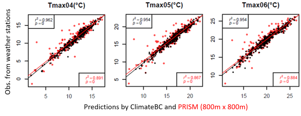
The scale-free feature considerably improves the accuracy of climate variables. For example, ClimateBC (a subset of ClimateNA) predictions of monthly maximum temperatures have much stronger relationships with observations from weather stations (Figure 8).

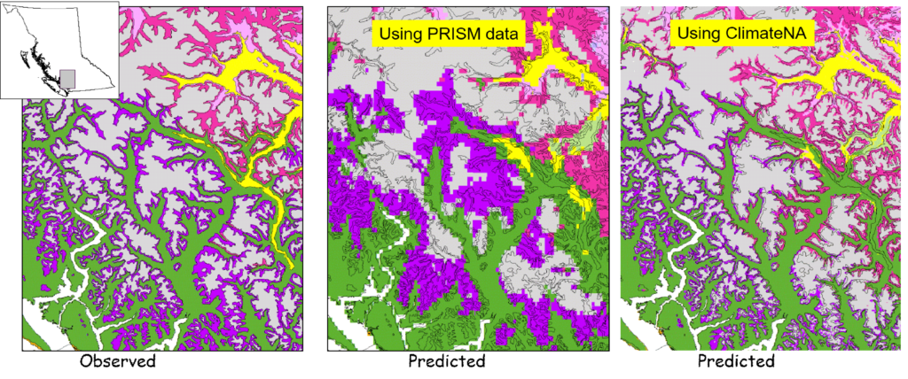
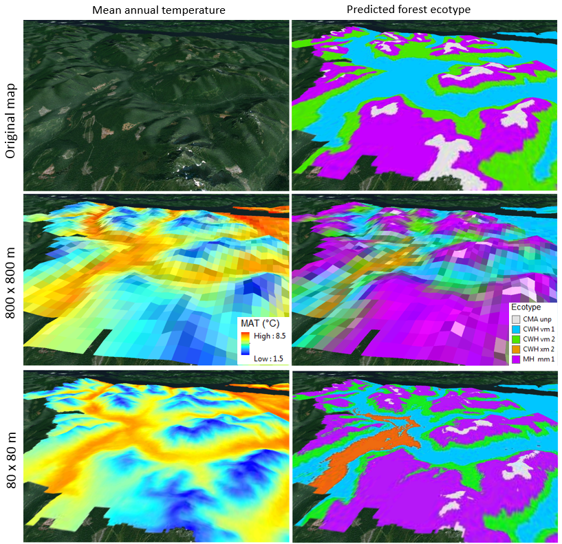
Scale-free climate data improve the prediction accuracy of ecological models. Climate variables of ecological sample plots predicted by ClimateNA or ClimateAP can better represent climatic conditions of the specific locations of the sample plots, thus can help to build more accurate ecological models. Figure 9 demonstrates an evident improvement in the prediction accuracy of an ecological niche model modeling the biogeoclimatic zones in British Columbia.

ClimateNA and ClimateAP can generate spatial climate data surfaces at any spatial resolution. The output spatial resolution of the climate variables is determined by user’s input dataset. This is particularly important for regional or local applications of ecological models, as a finer spatial resolution is often required to reflect the situation meaningful for practical applications (Figure 10).

5.2. All-in-one package

ClimateNA and ClimateAP integrate and downscale climate data for historical and Future years and periods. ClimateNA also integrates and downscales climate data for paleo periods (Figure 11). This prevents users from the need to obtain climate data from different sources with different climate variables with different data formats.

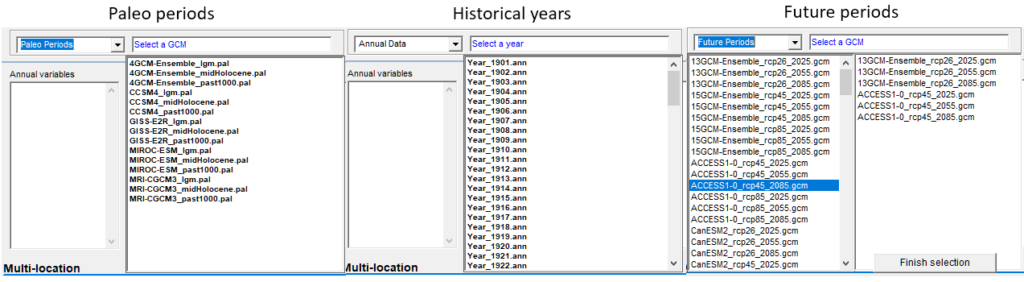
5.3. Multiple-location and multiple-GCM processing

ClimateNA and ClimateAP can process an almost unlimited number of locations in a single run. It can also generate climate data for multiple GCMs in a single run.

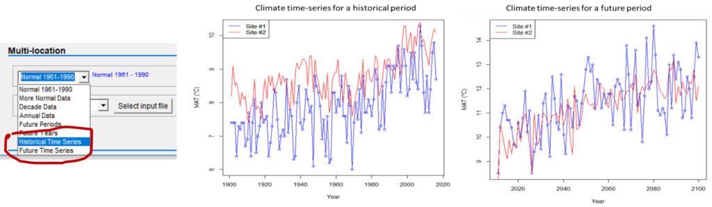
5.4. Time-series functions

ClimateNA and ClimateAP can generate time-series climate data for historical (1901-2019) or future years (2011-2100) for multiple locations in a single run. These functions can save users a tremendous amount of time.

5.5. Map-in and map-out capacity

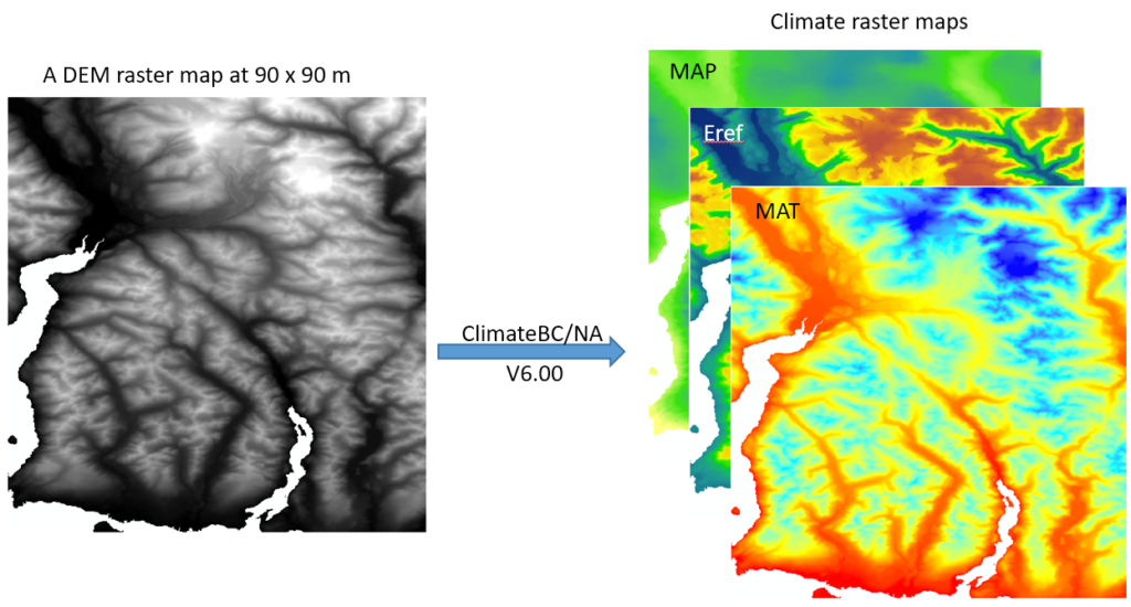
Since version 6.0, ClimateNA can read DEM raster file and generate climate variables in raster format for mapping. In previous versions, users need to convert a digital elevation model (DEM) to a spreadsheet file (i.e., a CSV file) as an input file, and also need to convert the output file to raster files. The new versions can directly read a DEM file in raster format and generate climate variables in raster format (as illustrated in Figure 13), which can be directly imported to a mapping software including R.

6. Web versions

Web versions of ClimateNA and ClimateAP are available to facilitate easy access to climate data for users dealing with a small number of locations. Users just need to click at the locations on Google Maps to obtain climate variables without the need to type in latitude, longitude, and elevation of the locations as they are automatically retrieved through the Google Map Services. The obtained climate data can be saved to a local computer.

The web versions also allow users to visualize the spatial patterns of major climate variables. Users can use Google Maps’ features to navigate and to zoom in or out around the locations of interest. The maps of the major climate variables can be downloaded in a picture or raster format.

In addition, the web versions serve as a platform to host the spatial data of forest ecosystems and species distributions under current and future climates. This feature has been widely used as a basis for foresters to develop forest adaptive strategies and as demonstrations of the impact of climate change on ecosystems and forest tree species in high school and university classes.

The web version of ClimateNA has two subsets, ClimateBC and ClimateWNA, to focus on regional interests (Figure 14). ClimateBC focuses on British Columbia. In addition to climate data, it hosts forest ecosystems and species distributions. ClimateWNA hosts several major forest tree species in western North America.

The web version of ClimateAP has five subsets, ClimateChina, ClimateLaos, ClimateMalaysia, ClimateMyanmar, and ClimateTaiwan, for different economies (Figure 13). Each hosts climate surfaces and ecosystem projections of its own region.

7. Spatial data

Pre-generated spatial climate data in raster format for entire North America. The datasets were produced by AdpatWest, which includes climate data for reference and future periods with many GCMs.

By Tongli Wang, Climate Modelling and Forest Applications is licensed under Creative Commons <CC BY-NC-ND 4.0> License