7 Topic 4.3. Introduction to Climate Response Functions
Lecture videos:
Contents
1. Overview
2. Definition
3. Response functions with a single variable
3.1. Objectives
3.2. Provenance test and climate data
3.3. Finding populations for future climates
3.4. Anchor points
4. Response functions with multiple climatic variables
4.1. Function
4.2. Response surface and function parameters
4.3. Model interpretation
5. Multiple response functions
5.1. Objectives
5.2. Putting multiple response curves on the same plot
5.3. Comparisons among multiple response curves
5.4. Limitations
6. Universal response functions
6.1. Objectives
6.2. Function
6.3. Features
1. Overview
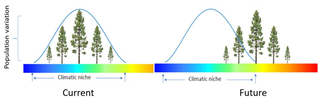
The concept of the population response function is relatively new in ecology. It was first introduced to model forest trees by Dr. Rehfeldt in 1999. It can predict the mismatch at the population level individually (vertically in Figure 1). It can also predict the mismatch at the species level integratively if an adequate number of populations are modeled (both vertically and horizontally in Figure 1). In addition, the climatic niche model by using response functions represents the fundamental niche of the species instead of the realized niche as modeled using presence-absence data.
2. Definition
A population response function describes the response of a population to the change of environmental conditions. It represents the environmental effect on the population. It also reflects the plasticity of the population over a range of environmental conditions.
This is contrasting to genecology functions or transfer functions, which are to model among-population variations in performance along environmental gradients of population origins. They reflect genetic variation in populations associated with environmental factors. A common feature of these two kinds of models is that they both are built based on provenance tests.
A typical linear and quadratic population response functions can be written as:
Y = a + bx [1]
Y = a + bx + cx2 [2]
Where, Y is the performance of a population; x is one (or more) environmental variable of test sites; and a, b, and c are parameters to be estimated to fit the model.
Similar to a genecology function, a response function can be with geographical variables (e.g., latitude, longitude, or elevation), or climatic variables (e.g., temperature and precipitation). Climatic variables are increasingly used as they have many advantages over geographical variables, particularly for predicting the impact of climate change on forests. Up to date, all response functions are built with climatic variables.
3. Response functions with a single variable
3.1. Objectives
A single climatic variable often plays a dominant role in affecting the performance of populations. For simplicity, we can build a response function with just one climatic variable. With a single climatic variable, a response function can reflect a simple linear relationship with a single climatic variable. It can also be built with a polynomial function, such as a quadratic, a cubic function. A quadratic function showing a bell-shape response curve is most commonly used as most climatic variables have an optimal range suitable for a plant species to grow.
3.2. Provenance test and climate data
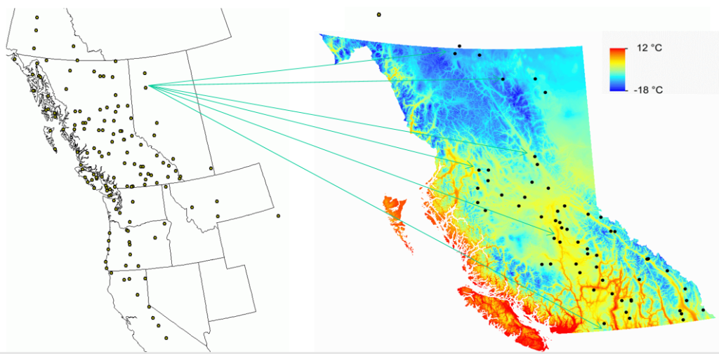
Let’s use the same provenance test shown in Figure 2 to demonstrate response functions. In the provenance test, each population was planted at multiple test sites. After 20 years of growth under different environmental conditions, the population showed substantial differences in performance among the test sites.
3.3. Finding populations for future climates
After we obtained climate data from ClimateNA, we can develop a response function for this population to represent the effect of temperature on the tree height of the population. As shown in Figure 3, the response function predicts the performance of the population Pop1 in different temperatures with its optimal performance around its local temperature. With an increase in temperature by 2°C due to climate change, the predicted productivity is predicted to drop substantially. We need to find populations that perform better in a warmer climate. Ideally, we may found populations that can perform well over a broader range of temperatures covering both the current and future climates.

3.4. Anchor points
Most provenance tests have a limited number of test sites due to the high cost and availability of planting sites. Also, due to a large number of provenances, there is no enough space to include all provenances. As a result of these situations, some provenances are often not tested at some extreme climatic conditions and make it is difficult to build an effective response function. For the latter case, a genecology function can be used to predict the performance of the missing populations at the site where the genecology function is built for. The predicted values are called anchor points as they play a role to anchor the curve down at the end of the species range. Details are described in Wang et al. (2006).
4. Response functions with multiple climatic variables
4.1. Function
A single variable is often not sufficient to explain the variation in the performance of a population across different environmental conditions. In those cases, two or more environmental variables are needed to be included in the model to increase its explanatory power. Then, the formula of a quadratic response function with multiple variables becomes:
Y = b0 + b1x1 + b2cx12 + b3x2 + b4cx22 + …
Where, Y is the performance of a population; x1, x2, …, are the climatic variables; and b0, b1, b2, …, are parameters to be estimated to fit the model.
4.2. Response surface and function parameters
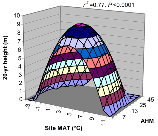
We use the dataset from the same provenance test for lodgepole pine to illustrate the response surface. A quadratic response function is built with two climatic variables, mean annual temperature (MAT) and annual heat-moisture index (AHM), as predictors. The response surface represents the response function is shown in Figure 4. The parameters estimated for the response function and the significance of the predictors are listed in Table 1.
Tabe 1. Parameters estimated and significance of the predictors
| Estimate | Std. Error | t value | Pr(>|t|) | Significance | |
| (Intercept) | 1.731036 | 1.758753 | 0.984 | 0.3298 | |
| MAT | 2.231324 | 0.511851 | 4.359 | 6.68E-05 | *** |
| AHM | 0.303606 | 0.145037 | 2.093 | 0.0415 | * |
| MAT^2 | -0.24298 | 0.05008 | -4.852 | 1.28E-05 | *** |
| AHM^2 | -0.00755 | 0.003411 | -2.214 | 0.0315 | * |
| MAT*AHM | -0.0126 | 0.028548 | -0.441 | 0.6608 |
4.3. Model interpretation
The information from the response surface shown in Figure 4 and the parameters estimated in Table 1 shows that MAT plays a dominant role in affecting the performance of the population, while AHM also significantly contributes to the model. However, the interaction between MAT and AHM does not significantly contribute to the model. In total, the model explains 77% of the total variation in tree height of the population among all the test sites. The model is highly accurate at P < 0.0001.
The response surface also shows: 1) this population can grow within the range between -3°C and 11°C for MAT and between 5 and 45 for AHM, but slightly varying depending on each other (i.e., climatic niche of this population); 2) the optimal climatic condition for this population is a combination between MAT at around 5°C and AHM at about 13; however, 3) the population can grow well between 3°C and 7°C for MAT and between 10 and 20 for AHM.
5. Multiple response functions
5.1. Objectives
A population response function built for a population reflects the characteristics of the given population. In other words, the function does not represent the responsive nature of other populations. To understand the difference among populations in this regard, we need to build response functions for other populations individually and then make comparisons among them. If there are a sufficient number of populations having response functions built, they can provide an overview of the response to climate at the species level.
5.2. Putting multiple response curves on the same plot
After response functions are built for multiple populations, to make comparisons among the response functions is important. Putting the response curves on the same plot is the most straightforward approach to make such a comparison. However, it is difficult to do so if the response functions are built with two or more climate variables. A solution for this is only to compare the response against the dominant variable while keeping the other variables constant or at their optimums. Figure 5 shows multiple response curves against MAT on the same plot while keeping AHM at its optimum for lodgepole pine.
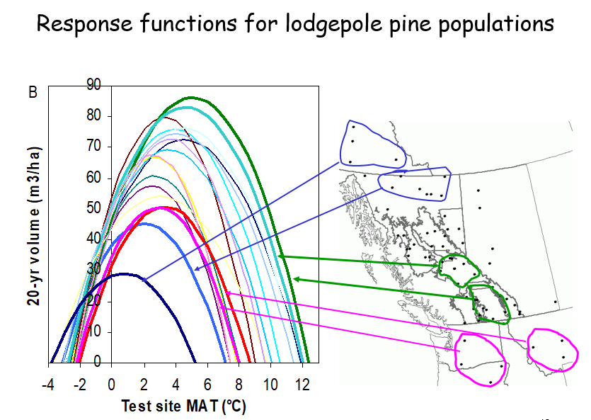
Figure 5. Comparisons in response curves among populations of lodgepole pine in BC. Image by Tongli Wang under CC BY 4.0.
5.3. Comparisons among multiple response curves
Through comparisons among the response curves shown in Figure 5, the following results can be drawn:
- 1) Lodgepole pine can grow between -4°C and 12.5°C in MAT (broader than Pop1).
- 2) Northern populations outperform other populations in a very cold environment at the could end of the species range, but grow much slower in all other environments.
- 3) Populations from the warmer locations in the south are not performing better than many other populations in warmer conditions.
- 4) The best performing populations are from the center of the distribution in southern BC. Those populations not only outperform other populations in most environments but also have a broader adaptational range.
- 5) An increase in temperature due to climate change will improve the performance of the northern populations to some extent; it will not make them outperform the central populations. To count on the increase in productivity in the north to compensate for the productivity loss in the south due to global warming is not realistic.
- 6) Thus, to mitigate the impact of climate change on the productivity of this species, we need to migrate the central populations to the north when the climate becomes suitable.
These results drawn from the comparison provide a scientific basis for developing adaptive forest management strategies.
5.4. Limitations
Response functions predict the response of populations to the change in environmental conditions, primarily climatic conditions. It is probably the most straightforward approach for understanding the impact of climate change on the performance of populations and for developing forest adaptive strategies. However, it has the following two limitations:
- 1) A response function developed for a population only reflects the responsive nature of the given population. Thus, it may not be able to represent other populations.
- 2) A credible response function can only be developed if a population is tested at multiple test sites across a wide range of climatic conditions. Most provenance tests comprise only a small number of test sites located in central distribution areas. Genecology functions or transfer functions are a better choice for these cases.
6. Universal response functions
6.1. Objectives
Genecology functions and transfer functions represent variation in the performance of populations caused by their origin (genetic effect). In contrast, response functions explain the variation in performance in response to differences in climatic conditions among test sites (environmental effect). Both have limitations in practice applications; a genecology function or a transfer function built for a test site may not apply to other environments. Similarly, a response function developed for a population may not apply to other populations. A universal response function is developed by Wang et al. (2010) to overcome these limitations by integrating both the genetic effect and the environmental effect into one model, as illustrated in Figure 6.
Figure 6. Illustration of integrating genecology functions and response functions to build a universal response function.
6.2. Function
A universal response function is a combination of a genecology function and a response function. A genecology function can be written as
Y = b0 + b1x1 + b2x12
Where, Y is the performance of a population; x1 is one (or more) environmental variables of provenance; and b0, b1, and b2 are parameters to be estimated to fit the model.
A response function can be written as
Y = b0 + b1x2 + b2x22
Where, Y is the performance of a population; x2 is one (or more) environmental variable of test site; and b0, b1, and b2 are parameters to be estimated to fit the model.
Then, a universal response function can be written as
Y = b0 + b1x1 + b2cx12 + b3x2 + b4cx22 + b5x1x2
Where, Y is the performance of a population; x1 and x2 are as defined above; x1x2 is the interaction between x1 and x2; b0, b1, b2, …, b5 are parameters to be estimated to fit the model.
Figure 7 shows a universal response function built for lodgepole pine from Wang et al. (2010). As the complete model involves multiple variables, the response surface is produced based on the two most important climate variables for visualization.
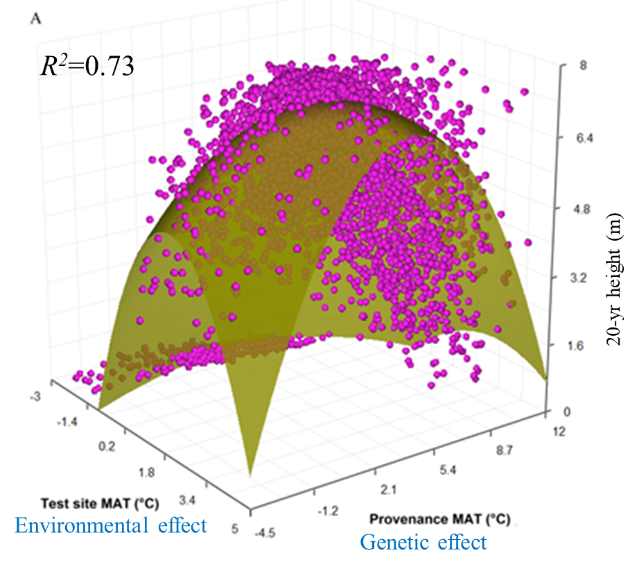
Figure 7. Response surface of a simplified universal function for lodgepole pine. Image by Tongli Wang under CC BY 4.0.
6.3. Features
Through the integration of both genetic and environmental effects into a single model, a universal response function has the following unique features:
- 1) A URF model can predict the performance of a population from any climate and planted at any climate. In other words, it can predict the performance of any population planted anywhere.
- 2) Model accuracy is improved. Genecology functions or transfer functions reflect the genetic effect among populations, while response functions describe the environmental effect. The URF model integrates both the environmental and genetic effects, thus improves the model accuracy. The simplified version of the URF shown in Figure 7 explains 73% of the total variation in population performance, while the full model accounts for 83% (Wang et al. 2010).
- 3) Environmental and genetic effects on population performance can be quantified and compared. By taking partial derivatives respect to site climate and provenance climate, respectively, the rate of change alone the site climate and provenance climate gradients can be calculated (Figure 8).
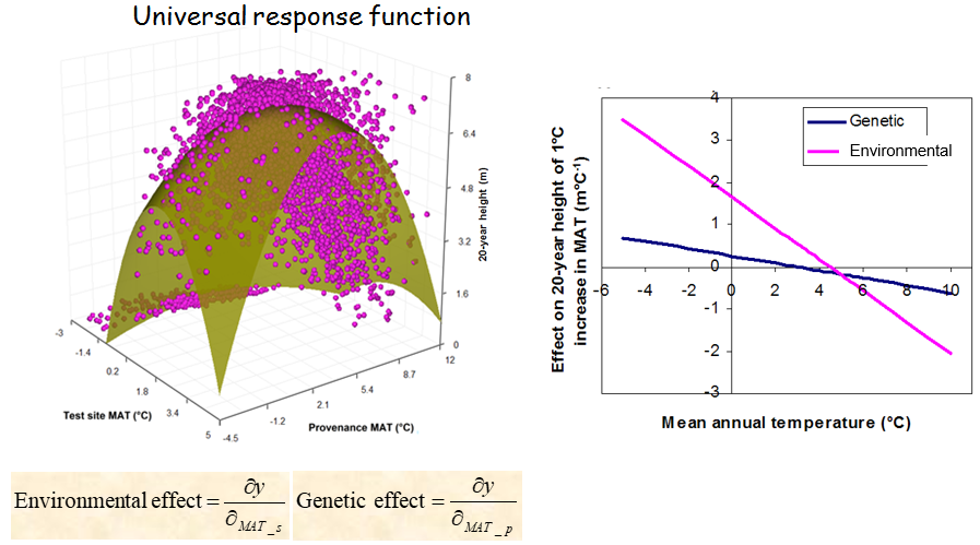
Figure 8. URF response curve and effects of genetic and environmental effects on population performance. Image by Tongli Wang under CC BY 4.0.
- 4) It relaxed the requirement for sample size. The URF takes better use of information obtained from a provenance test by including both site and provenance climates into the model; thus, it can achieve the same model accuracy by using much smaller sample sizes (Figure 9).
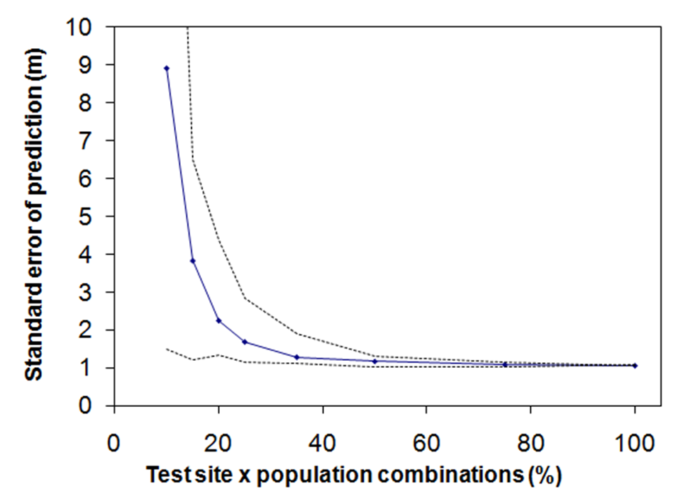
Figure 9. genecology functions developed at six test sites from cold to warm climates. Image by Tongli Wang under CC BY 4.0.
- 5) A URF can identify optimal provenances for any planting sites. By setting the partial derivative function to zero, the optimal values of the provenance climate can be determined, which can be used to locate the optimal provenances. Through comparisons of the difference in performance between local and optimal provenances, adaptational lag can be assessed (Hu et al. 2019).
- 6) A URF can be used to model the climatic niche of a species. The output of a climatic niche model is usually either in binary format (presence and absence) or in probability (0 ~ 1), while A URF is usually built with growth traits. It can be consider as absence if growth is zero and the rest as presence. As there is no interspecies interaction in common garden experiments for provenance tests; thus, the climatic niche predicted by a URF can be regarded as a fundamental niche, which is more relevant for the use in assisted migration (to be discussed in later topics). In addition, URF predictions covering the information for both climatic niche and growth potential. Figure 10 shows the climatic niche, growth potentials using local and optimal provenances of lodgepole pine for the current and future periods.
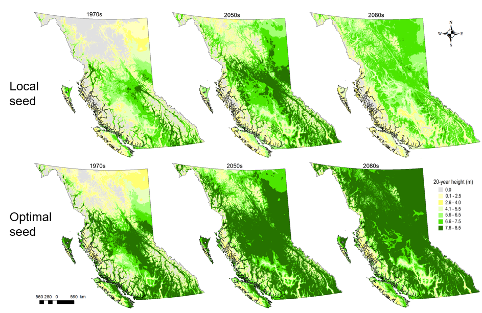
Figure 10. Climatic niche, growth potentials using local (the upper panel), and optimal (the lower panel) provenances of lodgepole pine for the current and future periods. Image by Tongli Wang under CC BY 4.0.

By Tongli Wang, Climate Modelling and Forest Applications is licensed under Creative Commons <CC BY-NC-ND 4.0> License
