Part 1 – Project Setup
Chapter 1.2 – Setting Up Images
Overview
In this chapter, the aim is to ensure that the images captured by the RPAS are ready for processing in MetaShape. A MetaShape project will be created into which the supplied RPAS images will be imported and then aligned to generate a spare point cloud with tie points.
MetaShape Project Setup
Download the RPAS images here. Create a folder called Multi-spectral in the Documents folder on your workstation. Open the Multi-spectral folder, create a sub-folder called Images and unzip the downloaded images into this sub-folder. You will have to remember the location of the Images folder. Ensure that all 4,465 images are present and note that each numbered image has a suffix (e.g. IMG_0131_1.tif). The suffix ( _x, where x = 1 through 5) indicates the multi-spectral band of each photo.
| Spectral Band Number | Spectral Band Characteristics |
| 1 | Blue (465 to 485 nm) |
| 2 | Green (550 to 570 nm) |
| 3 | Red (663 to 673 nm) |
| 4 | Near Infrared (820 to 860 nm) |
| 5 | Red Edge (712 to 722 nm) |
The full manual for the MicaSense RedEdge M multi-spectral sensors is available here.
From the Start menu, find and launch Agisoft MetaShape Professional.
Import Photos
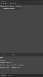
Each of the five multi-spectral bands will need to processed separately in their own chunk. Ensure that your’re in the Workspace tab (Fig. 1 bottom left of screen), select Add Chunk (Fig. 1) and rename the chunk to Blue.
From the Workflow menu, select Add Photos, navigate to the Images sub-folder and in the Search Images box enter *_1 to find only the blue spectral band images. Select all images and click Open. From the Add Photos dialogue box, select Single Cameras and click OK. Your should now see a view similar to Fig. 2 although you may need to select Show Cameras first.
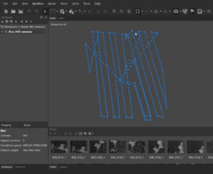
Select the Reference tab (bottom left of screen), to view all of the photos along with their longitude, latitude, altitude and estimated accuracy. Each photo thumbnail is also visible in the bottom Photos pane and a full resolution image can be opened by double-clicking the thumbnail.
In the main Model window, all of the image centers (principal point) are shown lined up according to how the RPAS flew the pre-programmed image acquisition mission (Fig. 2). The ball in the center of the Model window is used to rotate and spin the model in the X, Y and Z axes using the left mouse button. The right mouse button moves the model around while zooming in/out is done using the scroll-wheel on a mouse or by sliding two fingers on a touch pad.
Spin the model 90 deg from a top-down map view to a profile view as per Fig. 3. Notice that in addition to all the photos taken while the RPAS was at the operating altitude (approximately 68 to 93m), there is also a “column” of points extending down to the ground. These represent the photos that were taken while the RPAS was taking off and landing and need to be removed prior to any further processing.
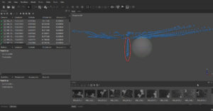
The best way to filter out these points is to search in the Altitude column of the Reference pane for values that are lower than the altitude at which the mission was flown (i.e. lower than ~68m). The easiest way to accomplish this is to sort the Altitude column from lowest to highest, select all photos from the lowest altitude to ~65m, right-click, select Remove Cameras and click Yes in the confirmation box.
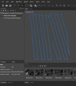
Press 0 (zero) to rotate the images back to map view. You’ll notice there are several “transit” lines (non-parallel to the flight lines) which are due to the RPAS transitioning between the take-off/landing and the starting point of the mission. These images do not represent data that should be processed. Manually select them in the list of cameras and remove them in a similar way as described above. When finished, you should end up with between 400 and about 500 cameras and a pattern similar to Fig. 4.
Assess Image Quality
The next quality assurance step is to assess the quality of the input photos. MetaShape checks basic photo attributes such as motion blur, focus, contrast and exposure. In the bottom Photo pane, switch to Details view, right-click on one of the photos , select Estimate Image Quality…, select All Photos then OK to see the quality score. Scores range from 0 (unacceptable) to 1.0 (perfect) and any photos below 0.6 should not be included in further processing and removed.
Adjust Coordinate System
At this stage, it is important to adjust the coordinate system of the photos to match that of the coordinate system of the ground control points (GCPs). The coordinate system that the GCPs were collected in is NAD83(CSRS) UTM Zone 10N with the CGVD2013 geoid. To adjust the photo centers, in the Reference pane click on the Convert icon, and from the Coordinate System drop down, select NAD83(CSRS) / UTM zone 10N + CGVD2013 height (EPSG::6653) and click OK. Note that the photo coordinates have now been updated to Easting, Northing and an altitude relative to the CGVD 2013 geoid.
Aligning Photos
So far, the software only knows where the center of each photo should be in absolute space (i.e. the coordinate system established in the previous step). It doesn’t yet know how all the overlapping photos connect or fit together. This is the purpose of the alignment function in MetaShape. Aligning photos is based on a computer vision concept called Structure from Motion.
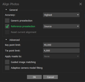
From the Workflow menu, select Align Photos, adjust the parameters to match Fig. 6 below and click OK.
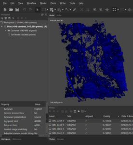
After a few minutes, the sparse point cloud showing the key tie points is generated and the view should look similar to the one below.
Save the project by accessing the File menu, selecting Save As…, naming it and clicking OK.
