Overview

Following the creation of a sparse 3D point cloud (i.e. tie points), the steps below outline the creation of dense 3D point cloud and the means of filtering out erroneous points.

Dense Point Cloud

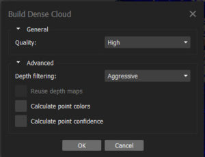
From the Workflow menu, select Build Dense Cloud… The Quality setting is directly dependent on available computing power. Reference this document to determine the suggested highest quality level based on the hardware being used. Set the quality as high as possible given your hardware configuration, as this ensures that the maximum number of pixels will be correlated in 3D space. Be aware that the higher the quality setting, the longer the processing time. Consider using lower setting for large data sets (i.e. several hundred photos). Suggested settings are shown below;

Maximum Density Cloud

The approximate maximum number of points in a dense cloud is calculated by multiplying the number of megapixels of the camera (e.g. 12 megapixel images are 4000 x 3000 pixels thus contain 12 million pixels each) by the number of images (496 in this data set) which equals 5,952,000,000! It is impossible to correlate all points and thus the actual number of pixels in a point cloud is generally only a fraction of the total possible (0.1 to 5%).

The resulting dense point cloud is similar to the key point, low density cloud but it contains exponentially more 3D information (aboutt 25 million compared with 500,000). The result should look similar to the screenshot below, but don’t be concerned if the number of points doesn’t match exactly.

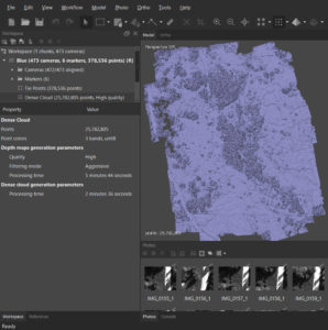
Although from certain perspectives, the dense cloud may look like a “solid” surface, it’s still just a collection of pixels positioned accurately in 3D space based on the GPS coordinates of the center pixel of each image. Due to the addition of GCPs, the accuracy of the location of any pixel was improved from +3m to about 1.5cm.

The next step is to filter any spurious points or outliers which are not representative of the surface being modeled.

Filter Dense Cloud

There are a number of different approaches to filtering points. They fall into two broad categories of semi-automated and manual. Here, only the manual method is demonstrated as it is the most selective and best applied to specific areas.

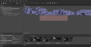
The general process involves rotating the dense cloud to identify individual points or groups of points that are not likely to be representative of the surface being modeled (e.g. points floating several tens of meters above the vegetation or any points below the “surface” of the field). Once points have been identified, the Selection (Rectangle, Circle or Free-form) is used to highlight the suspected outlier and pressing the Delete key on the keyboard removes them.

This is an iterative process and done well, greatly improves the chances of generating a quality 3D surface, which is the next step. See below for a sample of outlying points selected using the rectangle selection tool.

Adjust Region

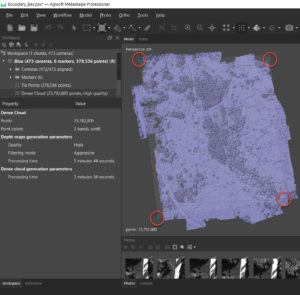
On your screen, you may notice the faint boundaries of a rectangle surrounding the dense cloud. This is the Region and defines the outer boundaries of the data set. It appears slightly tilted relative to the points being modeled. This can be adjusted as follows;

1. From the Model menu, open Transform Region and select Rotate Region
2. Using the “Track Ball”, adjust the angle of the region to match that of the dense point cloud as closely as possible.
3. Use the other Transform Region tools from the drop-down menu including Move Region, Resize Region and Reset Region.

Refer to the next Chapter for the creation of a digital surface model (DSM).