Part 2 – Generating 3D Maps
Chapter 2.2 – Digital Elevation Models
Overview
Once the 3D dense point cloud is generated, the next step is to create an accurate digital elevation model (DEM), digital surface model (DSM) or digital terrain model (DTM).
Before proceeding, be sure to save the project.
Building a DEM
A digital elevation model is a raster image (pixels, arranged in rows and columns) with each pixel representing an elevation. If the model represents elevations of the ground along with heights of structures such as buildings and trees, it can be referred to as a digital surface model (DSM). If the elevations only represent the ground or the bare earth, the model is referred to as a digital terrain model (DTM). The general term describing any type of raster elevation surface is digital elevation model (DEM).
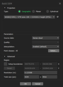
From the Workflow menu, select Build DEM…. The dialogue box settings are described below.
Projection Type can be set according to other data sets that you’d like this DEM to geographically coincide with.
Source data allows a choice between using the Sparse Cloud, Depth Maps, or Dense Cloud as the source of elevation data. The Sparse Cloud should never be used as it is the least accurate representation of elevation. The main difference between Depth maps (if available) or Dense Cloud is that the latter is the truest representation of the surface but may have holes or gaps where elevation data may be missing due to sparse alignment between photos. The former represents a more continuous surface (assuming that interpolation or extrapolation was enabled when building the mesh), keeping in mind that the interpolated elevations are algorithmic guesses based on surrounding known elevations.
Interpolation can be Enabled (default) to fill holes or gaps in elevations, Disabled or an Extrapolation can be applied instead.
Point classes can be selected (if they have been previously created through classification) or All (default) classes will be used.
Region settings can be adjusted if necessary, affecting the output Resolution and Total size of the DEM.
Fig. 16 below shows the suggested DEM settings for this project and don’t worry if the Region values are slightly different.
To view the DEM, double click it in the Workspace pane which brings up a new Ortho tab in the main view.
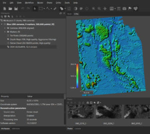
Note that the pixel resolution of the DSM in Fig. 17 is approximately 12.3cm. Also notice the clear demarcation of the lower and higher areas of vegetation.
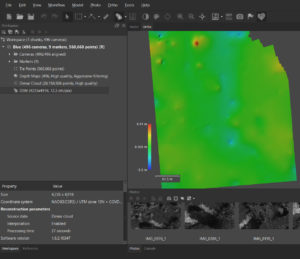
The alternate type of elevations surface that can be created is a digital terrain model (DTM). A DTM shows a statistical approximation of the ground or bare earth surface under vegetation and with all surface features (i.e. buildings and trees) filtered out. To build a DTM, the first step is to classify the dense point cloud.
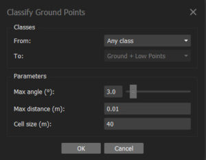
From the Tools menu, select Dense Cloud and then select Classify Ground Points….
Configure the parameters of the Classify Ground Points window as per Fig. 18 in order to generate three classes of points; Created (Never Classified), Ground and Low Point (Noise).
The next step is repeat the creation of the DEM, but this time specifying which class (Ground) to generate the elevation model with (Fig. 19).
Now that an accurate raster representation of the surface is generated, it can be used to create an orthophoto mosaic as described in the next Chapter.
