Overview

In this chapter, the goal is to add ground control points (GCPs) and use them to refine the relative and absolute orientations of the photos with reference to a real-world coordinate system.

Importing GCPs

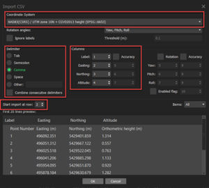
MetaShape will accept GCP files in a range of different formats and file types. For this exercise, the GCPs are in a comma-delimited format (CSV) which can be imported directly by MetaShape. In the Reference tab, select Import Reference, navigate to where your GCP file is stored (i.e. Boundary.CSV) and click Open. Adjust the Coordinate System, Delimiter and Columns as per Fig. 8, paying close attention to the Start import at row value (2 in this case) and click OK.

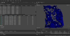
Click Yes to All when asked whether to “Create new marker?”. You should now see a view similar to Fig. 9 showing the initial locations of nine control points. If the markers flags are not visible in your image, click Show Markers in the main toolbar.

Placing GCP markers

In the Reference pane, notice the list of nine markers with their corresponding Easting, Northing and Altitude. Right-click on a Marker (e.g. 1) and select Filter photos by markers. Now, in the Photos pane along the bottom of the main display window, all the photos that GCP 1 appears in are shown.

Double-click the first photo and zoom in on the flag for GCP 1. It may be that the actual GCP is not visible in that photo! The flag can initially be several meters from the target due to the absolute positional error of the RPAS GPS. Select the next photo if that’s the case.

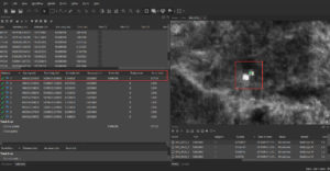
The goal is to left-click and drag the marker flag to the centre of the checkered GCP as per Fig. 10 below.

Notice now that the columns Error (m), Projections and Error (pix) now have values in them indicating the relative (pix) and absolute (m) error associated with placing that marker. In order to get a true sense of these errors, at least three GCPs need to be placed in a minimum of three photos (projections) followed by a least-squares adjustment. Double-click on the next photo and repeat the placement of the flag in the center of the target. Do this for at least six photos so as to build some redundancy. You may also find that the ground control targets are not easily visible in some photos.

Once you’ve placed GCP 1 into six photos, note the Error (m) and Error (pix) values. For example 0.897622m and 123.862 pixels, respectively. This means that even though we placed marker 1 in the center of the same target in all six photos, it is displaced by just over 123 pixels over the six photos. In an absolute sense, the coordinate value at the center of the ground control target, has an error of just less than 90cm over the six photos. These may seem like high error values, but recall that the last step is perform a least squares adjustment in order to distribute and minimize these errors. To do this, click the Update Transform icon. You should see a significant reduction in the errors now (e.g. 0.000678m and 0.199 pixels, respectively). Ideally, the goal would be an absolute error of less than 0.05m and a relative error of 0.5 pixels.

Now repeat the steps listed under the Place GCP markers section for the remaining eight GCPs. If some of the markers still yield errors higher than those specified above, refer to the section below.

Refining GCPs

Referring to Fig. 11 below, we can see that eight out of nine GCPs have been placed (GCP 9 has no data). Absolute errors range between 0.001884m and 0.012612m with an average of 0.006073m and relative errors range between 0.223 and 0.865 with an average of 0.604. These are acceptable results, but there are a few steps we can take to refine them further.

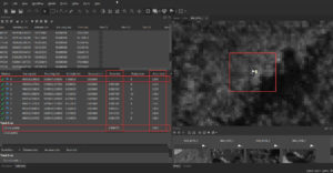
First of all, GCP 9 was not placed because, as can be seen from the right side of Fig. 11 above, the ground control point was not visible in the photos. In fact, as you may have already noticed, some of the GCPs were more difficult to locate in the photos than others. Lighting conditions, shadows, presence of vegetation are all factors in how easily a ground control target can be seen in a photo. It is better to leave out a GCP rather than try to forcefully place it when it can’t be properly identified and seen.

The next step to refine the results are to identify the specific photos in which a particular GCP marker has relatively high errors. The best approach is to sort the GCPs according to the Error (pix) column, right click on the top-most GCP and select Show Info…. In the window that opens, sort the Value column from highest to lowest and double click on the top-most value. This will immediately open the photo in which that marker has the highest relative error and the pop-up window can now be closed. There are now two options; 1) Try slightly moving the marker flag while keeping an eye on the Error (pix) column for that marker to see if the re-positioning of the flag reduces it, or 2) Right click on the marker flag and select Unpin Marker. Option one is valid only when the re-positioning of the marker flag towards the center of the GCP yields a lower error. If moving it away from the center reduces the error, then the only valid option is two.

Do this for each GCP trying to reduce the Total relative error (pix) below 0.5. Keep in mind to leave at least three projections for each GCP. Following these steps, the errors were reduced to 0.003598m (absolute) and 0.442 pixels (relative).

One final step can be performed to minimize any residual errors. This involves optimizing the camera parameters or performing a camera calibration. In the Reference pane, select Optimize Cameras, accept the default parameters and click OK. This step reduces errors due to lens and camera distortions including aspherical, tangential and radial. The final errors are now 0.001541m (absolute) and 0.308 pixels (relative). These are good results and the next steps of processing the images into the data products can now be taken.