Part 2 – Generating 3-D Maps
Chapter 2.1 – Dense Point Cloud
Overview
The steps below outline the creation of several 3-D map products starting with a high quality sparse point cloud following optimized photo aligment.
High Accuracy Alignment
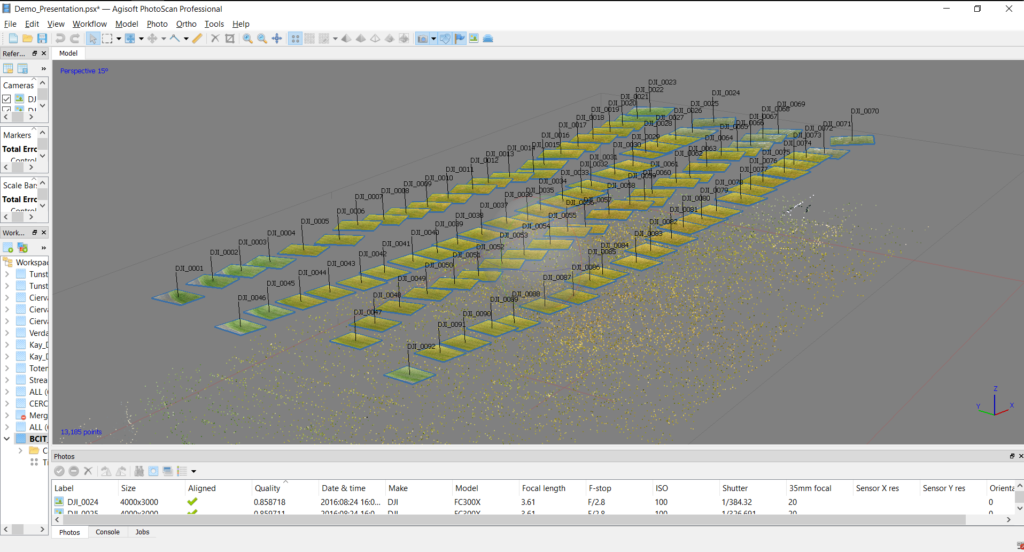
The low quality photo alignment identified approximately 13,185 key tie points between the overlapping photos. These points form the basis for stitching together all 92 photos together into a seamless mosaic.
Click Show Cameras, rotate the view and you should see a result similar to the screenshot below;
Recognizing the fact that all cameras exhibit some degree of distortion (e.g. radial, tangential, de-centering, etc.), it’s important to run an optimization which minimizes the effects of these distortions on the accuracy and precision of objects in the photos.
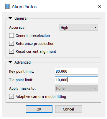
Click Optimize Cameras, accept the defaults and click OK. From Workflow, select Align Photos… and set the parameters according to the screenshot below;
Results of the high quality alignment (which may take about 15min to complete) are shown below with 372,566 key tie points identified. If the alignment is taking too long to complete (more than 20min), you can cancel the process and re-run it using lower quality settings and/or key/tie point limits.
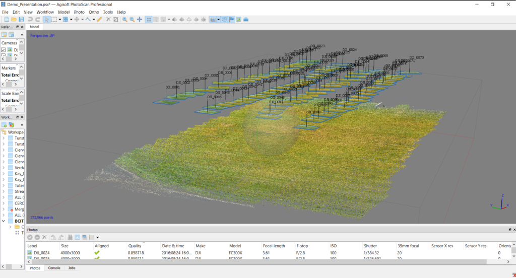
Photo Alignment
Sometimes, large data sets with complex, variable terrain (including trees), will result in misalignment of some photos. If any photos remain unaligned after the initial attempt, several steps can be taken to align them.
- Re-run Align Photos… using higher Key point and Tie point limits.
- Select all the unaligned photos (represented as dots instead of footprints in the model) from the Cameras folder under the BCIT_Field chunk, right-click, select Reset Camera Alignment then right-click again and select Align Selected Cameras,
- Running a higher quality alignment (if possible) can also help align photos.
Keep in mind that poor quality photos (quality index <0.6) or photos with very tall structures like trees or buildings that are significantly closer to the camera than the ground, may not align at all.
With the key points identified as accurately as possible, the next step is to locate as many of the remaining pixels in 3-D and generate the dense point cloud.
Dense Point Cloud
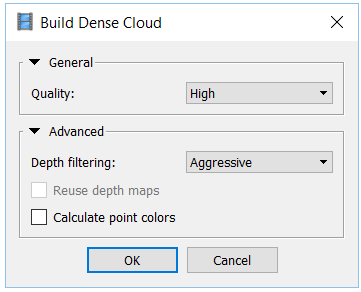
From the Workflow menu, select Build Dense Cloud… The Quality setting is directly dependent on available computing power. Reference this document to determine the suggested highest quality level based on the hardware being used. Set the quality as high as possible given your hardware configuration, as this ensures that the maximum number of pixels will be correlated in 3-D space. Be aware that the higher the quality setting, the longer the processing time. Consider using lower setting for large data sets (i.e. several hundred photos). Suggested settings are shown below;
Maximum Density Cloud
The approximate maximum number of points in a dense cloud is calculated by multiplying the number of megapixels of the camera (e.g. 12 megapixel images are 4000 x 3000 pixels thus contain 12 million pixels each) by the number of images (92 in this data set) which equals 1,104,000,000. It is impossible to correlate all points and thus the actual number of pixels in a point cloud is generally only a fraction of the total possible (0.1 to 5%).
The resulting dense point cloud is similar to the key point, low density cloud but it contains exponentially more 3-D information (39,184,432 3-D pixels!). The result should look similar to the screenshot below, but don’t be concerned if the number of points doesn’t match exactly.
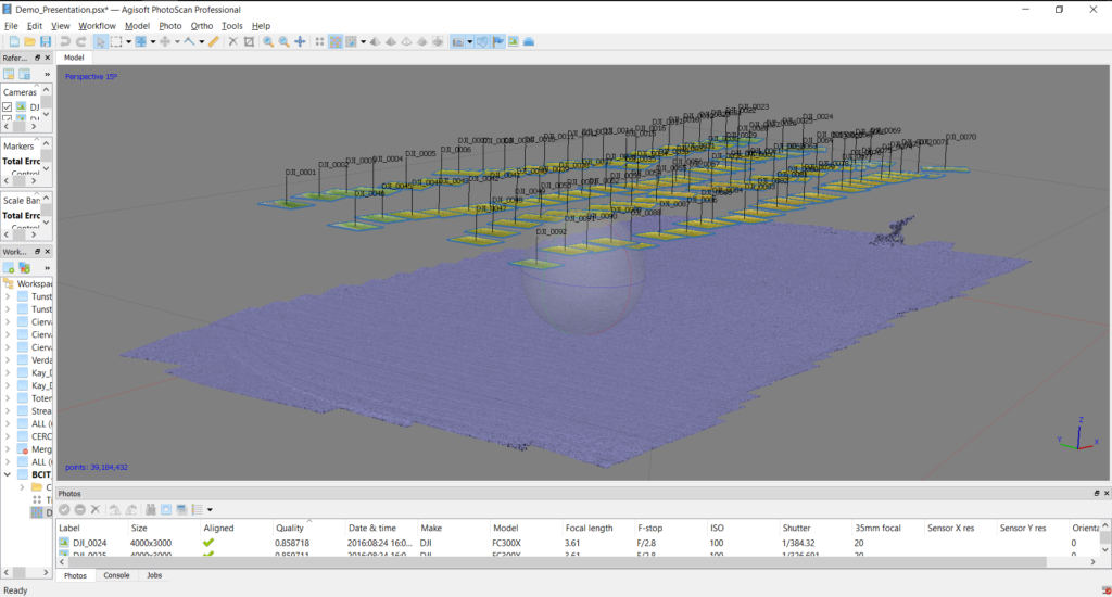
Although from certain perspectives, the dense cloud make look like a “solid” surface, it’s still just a collection of pixels positioned accurately in space based on the GPS coordinate of the center pixel of each image. Due to GPS error and any remaining distortions in the camera and lens, the actual position of any pixel may vary by upto +5m but the error usually much lower (+0.5m).
The next step is to filter any spurious points or outliers which are not representative of the surface being modeled in 3-D.
Filtering Dense Cloud Points
The type of surface greatly affects the ability and accuracy of filtering points. For example, the very level and flat playing field (except for the net) means that we shouldn’t expect much deviation from the “ground” at all. Conversely in heavily treed areas or where there is high frequency, large-scale changes in elevation (e.g. a boulder field), the precision with which outlying points can be effectively filtered declines significantly.
Filter Dense Cloud
There are a number of different approaches to filtering points. They fall into two broad categories of semi-automated and manual. Here, only the manual method is demonstrated as it is the most selective and best applied to specific areas.
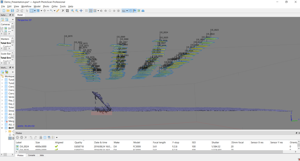
The general process involves rotating the dense cloud to identify individual points or groups of points that are not likely to be representative of the surface being modeled (e.g. points floating several tens of meters above the playing field or any points below the “surface” of the field). Once points have been identified, the Selection (Rectangle, Circle or Free-form) is used to highlight the suspected outlier and pressing the Delete key on the keyboard removes them.
This is an iterative process and done well, greatly improves the chances of generating a quality 3-D surface, which is the next step. See below for a sample of outlying points selected using the rectangle selection tool.
Adjust Region
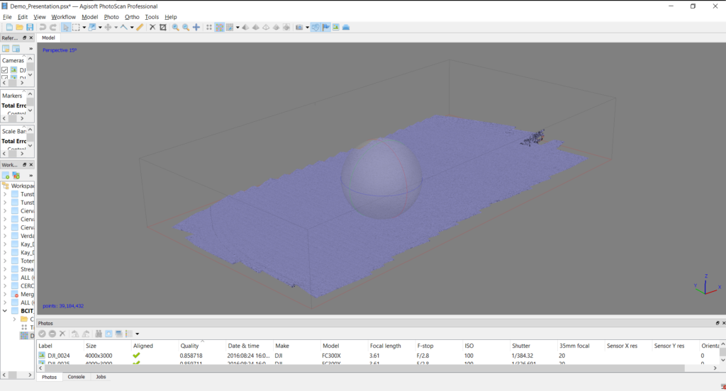
In the above screenshot, you may notice the faint boundaries of a rectangle surrounding the dense cloud. This is the Region and defines the outer boundaries of the data set. It appears slightly tilted relative to the points being modeled. This can be adjusted as follows;
- From the Model menu, open Transform Region and select Rotate Region
- Using the “ball”, adjust the angle of the region to match that of the dense point cloud as closely as possible.
- Use the other Transform Region tools from the drop-down menu including Move Region, Resize Region and Reset Region.
Refer to the next part for the creation of a 3-D mesh surface and textures.
