Overview

Once the dense point cloud is generated and filtered, the next step is create a continuous 3-D surface of the model. This process connects the discreet, 3-D pixels in the dense cloud with vector vertices, resulting in a “solid” without any gaps between points. In areas of the dense cloud where the points are relatively sparse, the surface can be either interpolated or extrapolated.

Generate Mesh

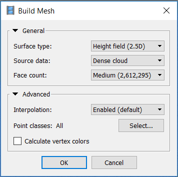
From the Workflow menu, select Build Mesh… to open the dialogue box. The parameter options are described below.

Surface Type can either be Arbitary (3-D) or Height field (2.5-D). The former retains 3-D pixel information for all points in the input point cloud. This surface type is suggested for modeling complex shapes with overhangs and images taken at low oblique angles (i.e. up to 30 deg tilt from Nadir). The latter results in a simpler surface as the height field is only interpreted as orthogonal to the horizontal plane (X or Y axis). No overhangs or such complex surface features are retained and thus the processing time is usually shorter.

The Input Surface can either be the sparse or dense point cloud (default).

Face Count is a measure of the final complexity of the surface. Higher face counts will result in more detailed morphology of features but sometimes at the expense of noise or artifacts because of the decimation process. This is also dependent on the hardware configuration.

Under the Advanced tab, the first setting is Interpolation (None, Enabled (Default), or Extrapolate). None will leave any small gaps or holes unfilled, Enabled will interpolate and fill small gaps and holes and Extrapolate will fill small gaps and holes using a simplified algorithm and also fill out the edge of the surface to the extents of the bounding box.

Point Classes defaults to All unless a previous step to classify the dense point cloud was performed.

The last option, Calculate Vertex Colors, determines whether the vertices will be colored using a photo pixel or not. This can be left unchecked because the following step of generating surface textures will handle this in a much more detailed way.

Set the options as per the screenshot below and proceed with generating the 3-D surface mesh.

Results of the 3-D mesh generation are shown in the screenshot below. As you can see, at first glance, it doesn’t look any different than the dense point cloud. The only minor difference is that the goalie net (right corner of the image) now looks more solid or extrapolated to the ground.

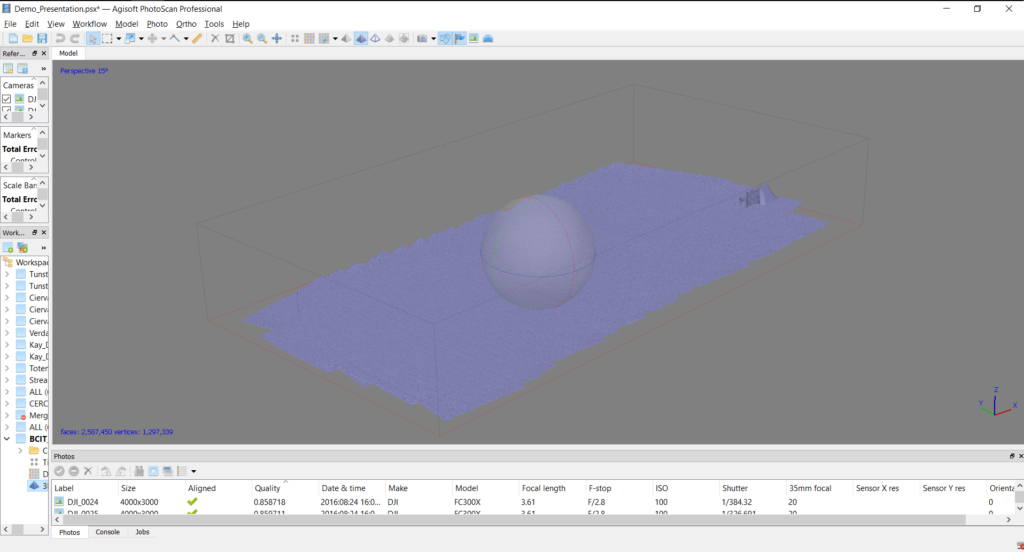
It is good practice to inspect the edges of the 3-D model. The number of key tie points is least along the edges of a model because that’s where the amount of photo overlap is lowest. It is always advisable to fly a project area at least one flight line and photo pair beyond the desired boundary. In this case, the edges actually look quite good.

Build Textures

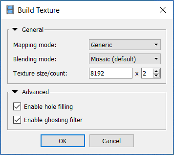
In order to add photo information to the 3-D mesh, it is necessary to generate textures which are then “draped” onto the model using several different algorithms. From the Workflow menu, select Build Texture…. The dialogue settings are described below.

Mapping mode determines what type of photo (e.g. Generic, Orthophoto, Adaptive Ortho, Spherical, or Single camera) is applied to the model. For the purposes of 3-D mapping, Generic or Adaptive orthophoto produce the best results.

Blending mode determines how the selected photo is applied to the 3-D model. The options are Mosaic (default), Average, Max intensity, Min intensity, Disabled. The default mode Mosaic is usually the best choice.

Texture/size count setting depends on the Mapping Mode and determines the resolution or detail of the texture. Count (if enabled) determines how the texture atlas is divided up. For example a setting of 4096 x 2 is the same as 8192 x 1 and generally higher values produce more detailed results.

Enable hole filling interpolates surrounding colors in areas where the texture atlas has a hole, generally due to there being insufficient points to correlate at least two photos.

Enable ghosting filter eliminates the chance of duplicate textures in areas where two or more textures overlap.

The settings below are suggested for this project.

The screenshot below shows photo textures applied to the 3-D mesh to give it a detailed, realistic look.

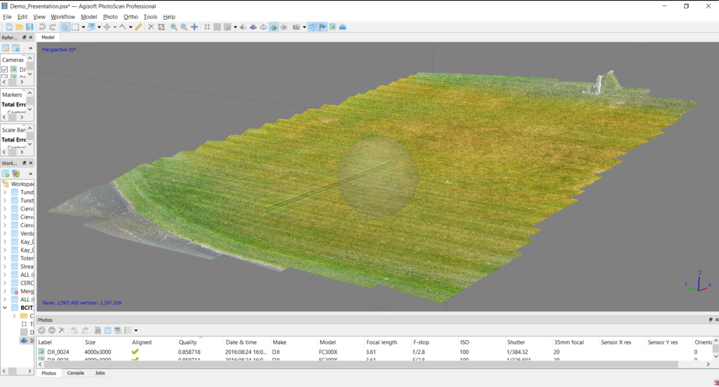
There is sufficient detail in the texturized 3-D mesh above that you can almost zoom into a 1:1 to scale and clearly see the blades of grass!

In the next part, the steps for creating a digital surface model and orthomosaic are described.