Chapter 21 Circuits and DC Instruments
163 21.3 Kirchhoff’s Rules
Summary
- Analyze a complex circuit using Kirchhoff’s rules, using the conventions for determining the correct signs of various terms.
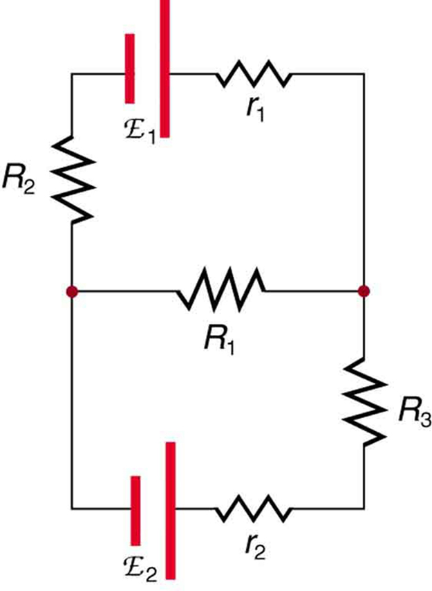
Many complex circuits, such as the one in Figure 1, cannot be analyzed with the series-parallel techniques developed in Chapter 21.1 Resistors in Series and Parallel and Chapter 21.2 Electromotive Force: Terminal Voltage. There are, however, two circuit analysis rules that can be used to analyze any circuit, simple or complex. These rules are special cases of the laws of conservation of charge and conservation of energy. The rules are known as Kirchhoff’s rules, after their inventor Gustav Kirchhoff (1824–1887).
Kirchhoff’s Rules
- Kirchhoff’s first rule—the junction rule. The sum of all currents entering a junction must equal the sum of all currents leaving the junction.
- Kirchhoff’s second rule—the loop rule. The algebraic sum of changes in potential around any closed circuit path (loop) must be zero.
Explanations of the two rules will now be given, followed by problem-solving hints for applying Kirchhoff’s rules, and a worked example that uses them.
Kirchhoff’s First Rule
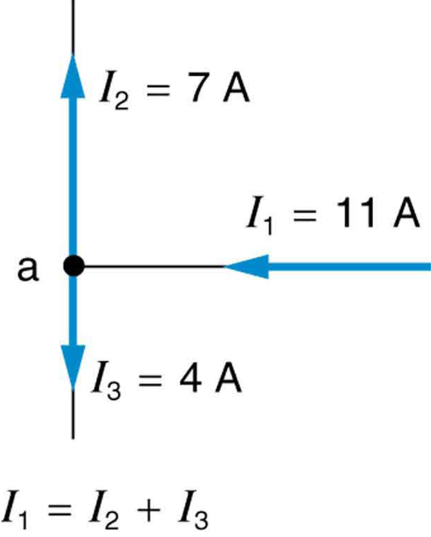
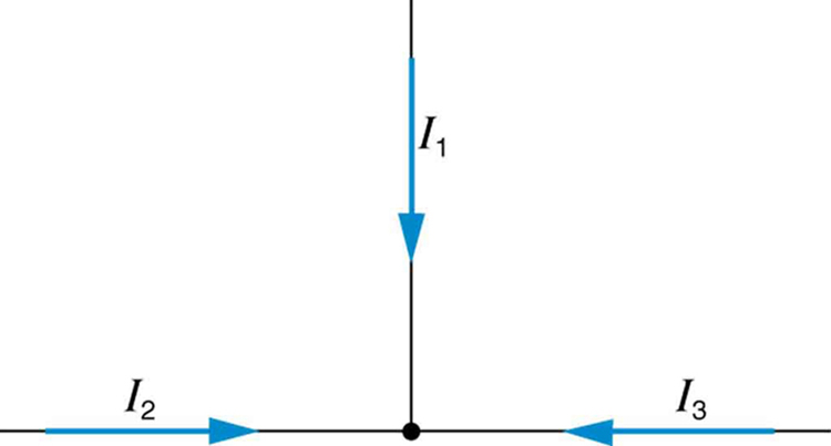
Kirchhoff’s first rule (the junction rule) is an application of the conservation of charge to a junction; it is illustrated in Figure 2. Current is the flow of charge, and charge is conserved; thus, whatever charge flows into the junction must flow out. Kirchhoff’s first rule requires that [latex]\boldsymbol{I_1 = I_2 + I_3}[/latex] (see figure). Equations like this can and will be used to analyze circuits and to solve circuit problems.
Making Connections: Conservation Laws
Kirchhoff’s rules for circuit analysis are applications of conservation laws to circuits. The first rule is the application of conservation of charge, while the second rule is the application of conservation of energy. Conservation laws, even used in a specific application, such as circuit analysis, are so basic as to form the foundation of that application.
Kirchhoff’s Second Rule
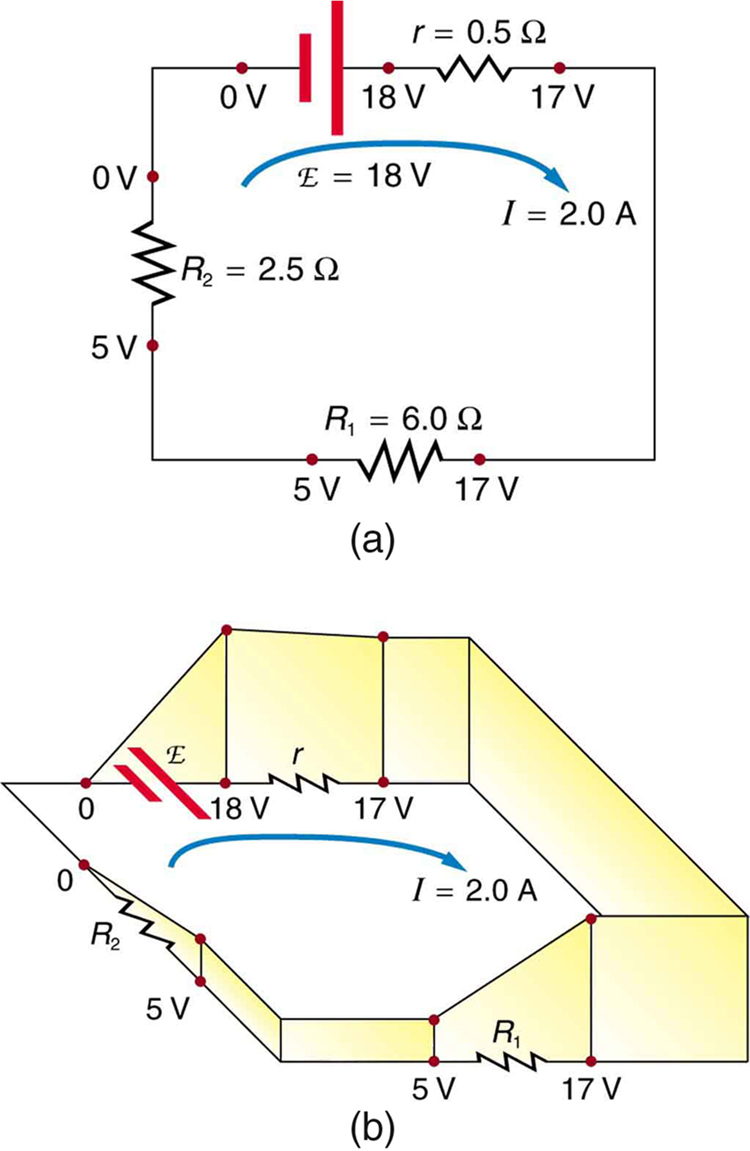
Kirchhoff’s second rule (the loop rule) is an application of conservation of energy. The loop rule is stated in terms of potential, [latex]\boldsymbol{V}[/latex], rather than potential energy, but the two are related since [latex]\boldsymbol{\textbf{PE}_{\textbf{elec}} = qV}[/latex]. Recall that emf is the potential difference of a source when no current is flowing. In a closed loop, whatever energy is supplied by emf must be transferred into other forms by devices in the loop, since there are no other ways in which energy can be transferred into or out of the circuit. Figure 3 illustrates the changes in potential in a simple series circuit loop.
Kirchhoff’s second rule requires [latex]\boldsymbol{\textbf{emf} - Ir - IR_1 - IR_2 = 0}[/latex]. Rearranged, this is [latex]\boldsymbol{\textbf{emf} = Ir + IR_1 + IR_2}[/latex], which means the emf equals the sum of the [latex]\boldsymbol{IR}[/latex] (voltage) drops in the loop.
Applying Kirchhoff’s Rules
By applying Kirchhoff’s rules, we generate equations that allow us to find the unknowns in circuits. The unknowns may be currents, emfs, or resistances. Each time a rule is applied, an equation is produced. If there are as many independent equations as unknowns, then the problem can be solved. There are two decisions you must make when applying Kirchhoff’s rules. These decisions determine the signs of various quantities in the equations you obtain from applying the rules.
- When applying Kirchhoff’s first rule, the junction rule, you must label the current in each branch and decide in what direction it is going. For example, in Figure 1, Figure 2, and Figure 3, currents are labeled [latex]\boldsymbol{I_1}[/latex], [latex]\boldsymbol{I_2}[/latex], [latex]\boldsymbol{I_3}[/latex], and [latex]\boldsymbol{I}[/latex], and arrows indicate their directions. There is no risk here, for if you choose the wrong direction, the current will be of the correct magnitude but negative.
- When applying Kirchhoff’s second rule, the loop rule, you must identify a closed loop and decide in which direction to go around it, clockwise or counterclockwise. For example, in Figure 3 the loop was traversed in the same direction as the current (clockwise). Again, there is no risk; going around the circuit in the opposite direction reverses the sign of every term in the equation, which is like multiplying both sides of the equation by –1.
Figure 4 and the following points will help you get the plus or minus signs right when applying the loop rule. Note that the resistors and emfs are traversed by going from a to b. In many circuits, it will be necessary to construct more than one loop. In traversing each loop, one needs to be consistent for the sign of the change in potential. (See Example 1.)
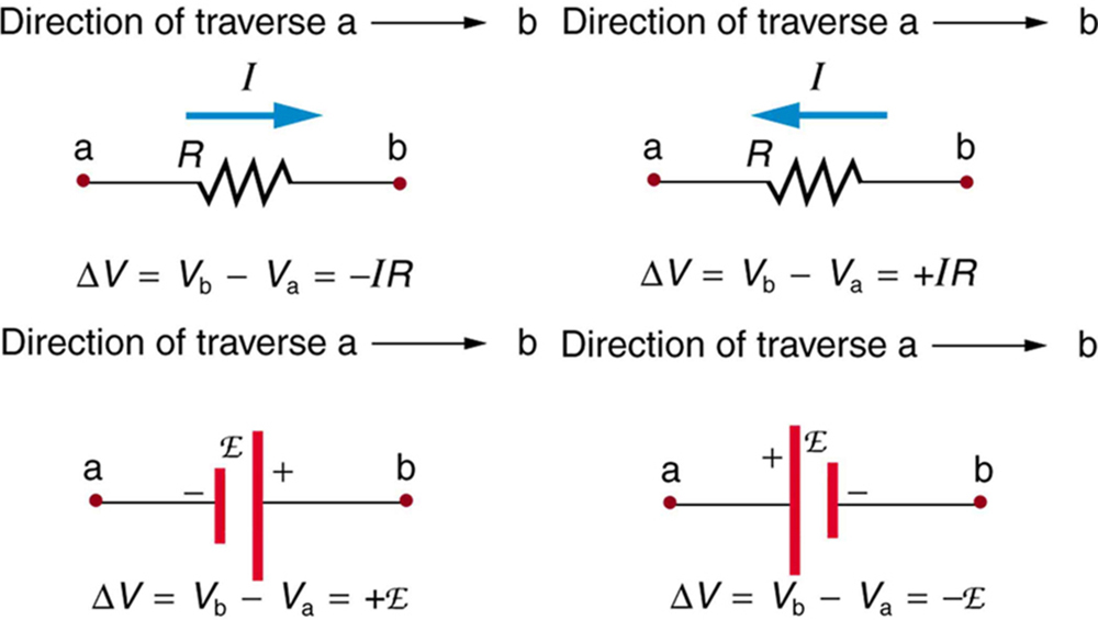
- When a resistor is traversed in the same direction as the current, the change in potential is [latex]\boldsymbol{-IR}[/latex]. (See Figure 4.)
- When a resistor is traversed in the direction opposite to the current, the change in potential is [latex]\boldsymbol{+IR}[/latex]. (See Figure 4.)
- When an emf is traversed from – to + (the same direction it moves positive charge), the change in potential is +emf. (See Figure 4.)
- When an emf is traversed from + to – (opposite to the direction it moves positive charge), the change in potential is −emf. (See Figure 4.)
Example 1: Calculating Current: Using Kirchhoff’s Rules
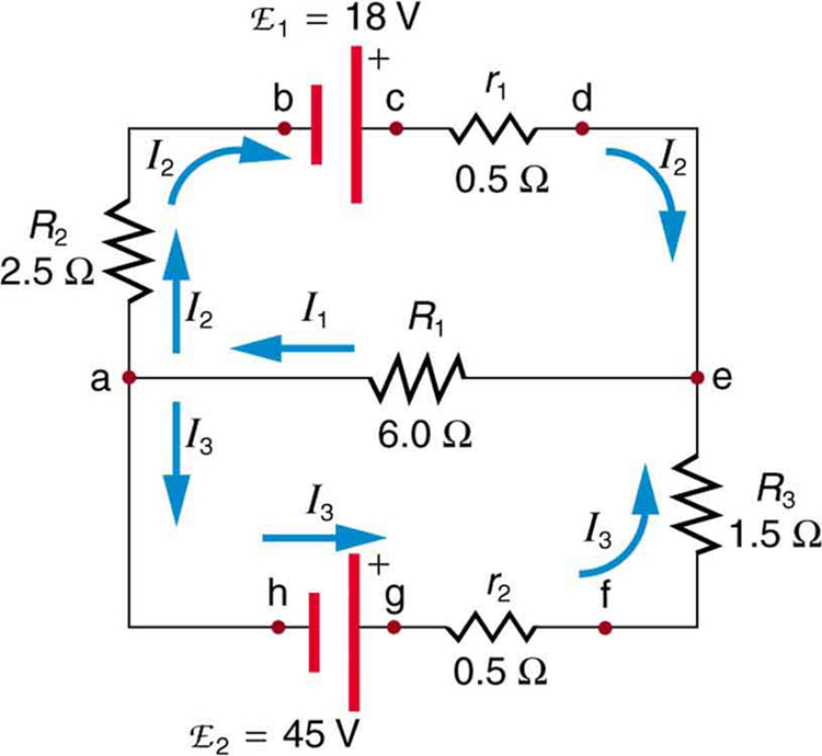
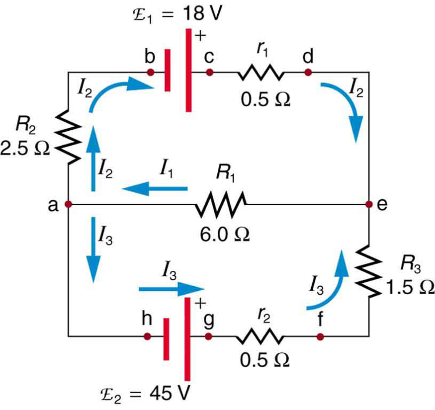
Find the currents flowing in the circuit in Figure 5.
Strategy
This circuit is sufficiently complex that the currents cannot be found using Ohm’s law and the series-parallel techniques—it is necessary to use Kirchhoff’s rules. Currents have been labeled [latex]\boldsymbol{I_1}[/latex], [latex]\boldsymbol{I_2}[/latex], and [latex]\boldsymbol{I_3}[/latex] in the figure and assumptions have been made about their directions. Locations on the diagram have been labeled with letters a through h. In the solution we will apply the junction and loop rules, seeking three independent equations to allow us to solve for the three unknown currents.
Solution
We begin by applying Kirchhoff’s first or junction rule at point a. This gives
since [latex]\boldsymbol{I_1}[/latex] flows into the junction, while [latex]\boldsymbol{I_2}[/latex] and [latex]\boldsymbol{I_3}[/latex] flow out. Applying the junction rule at e produces exactly the same equation, so that no new information is obtained. This is a single equation with three unknowns—three independent equations are needed, and so the loop rule must be applied.
Now we consider the loop abcdea. Going from a to b, we traverse [latex]\boldsymbol{R_2}[/latex] in the same (assumed) direction of the current [latex]\boldsymbol{I_2}[/latex], and so the change in potential is [latex]\boldsymbol{-I_2R_2}[/latex]. Then going from b to c, we go from – to +, so that the change in potential is [latex]\boldsymbol{+ \textbf{emf}_1}[/latex]. Traversing the internal resistance [latex]\boldsymbol{r_1}[/latex] from c to d gives [latex]\boldsymbol{-I_2r_1}[/latex]. Completing the loop by going from d to a again traverses a resistor in the same direction as its current, giving a change in potential of [latex]\boldsymbol{-I_1R_1}[/latex].
The loop rule states that the changes in potential sum to zero. Thus,
Substituting values from the circuit diagram for the resistances and emf, and canceling the ampere unit gives
Now applying the loop rule to aefgha (we could have chosen abcdefgha as well) similarly gives
Note that the signs are reversed compared with the other loop, because elements are traversed in the opposite direction. With values entered, this becomes
These three equations are sufficient to solve for the three unknown currents. First, solve the second equation for [latex]\boldsymbol{I_2}[/latex]:
Now solve the third equation for [latex]\boldsymbol{I_3}[/latex]:
Substituting these two new equations into the first one allows us to find a value for [latex]\boldsymbol{I_1}[/latex]:
Combining terms gives
Substituting this value for [latex]\boldsymbol{I_1}[/latex] back into the fourth equation gives
The minus sign means [latex]\boldsymbol{I_2}[/latex] flows in the direction opposite to that assumed in Figure 5.
Finally, substituting the value for [latex]\boldsymbol{I_1}[/latex] into the fifth equation gives
Discussion
Just as a check, we note that indeed [latex]\boldsymbol{I_1 = I_2 + I_3}[/latex]. The results could also have been checked by entering all of the values into the equation for the abcdefgha loop.
Problem-Solving Strategies for Kirchhoff’s Rules
- Make certain there is a clear circuit diagram on which you can label all known and unknown resistances, emfs, and currents. If a current is unknown, you must assign it a direction. This is necessary for determining the signs of potential changes. If you assign the direction incorrectly, the current will be found to have a negative value—no harm done.
- Apply the junction rule to any junction in the circuit. Each time the junction rule is applied, you should get an equation with a current that does not appear in a previous application—if not, then the equation is redundant.
- Apply the loop rule to as many loops as needed to solve for the unknowns in the problem. (There must be as many independent equations as unknowns.) To apply the loop rule, you must choose a direction to go around the loop. Then carefully and consistently determine the signs of the potential changes for each element using the four bulleted points discussed above in conjunction with Figure 4.
- Solve the simultaneous equations for the unknowns. This may involve many algebraic steps, requiring careful checking and rechecking.
- Check to see whether the answers are reasonable and consistent. The numbers should be of the correct order of magnitude, neither exceedingly large nor vanishingly small. The signs should be reasonable—for example, no resistance should be negative. Check to see that the values obtained satisfy the various equations obtained from applying the rules. The currents should satisfy the junction rule, for example.
The material in this section is correct in theory. We should be able to verify it by making measurements of current and voltage. In fact, some of the devices used to make such measurements are straightforward applications of the principles covered so far and are explored in the next modules. As we shall see, a very basic, even profound, fact results—making a measurement alters the quantity being measured.
Check Your Understanding
1: Can Kirchhoff’s rules be applied to simple series and parallel circuits or are they restricted for use in more complicated circuits that are not combinations of series and parallel?
Section Summary
- Kirchhoff’s rules can be used to analyze any circuit, simple or complex.
- Kirchhoff’s first rule—the junction rule: The sum of all currents entering a junction must equal the sum of all currents leaving the junction.
- Kirchhoff’s second rule—the loop rule: The algebraic sum of changes in potential around any closed circuit path (loop) must be zero.
- The two rules are based, respectively, on the laws of conservation of charge and energy.
- When calculating potential and current using Kirchhoff’s rules, a set of conventions must be followed for determining the correct signs of various terms.
- The simpler series and parallel rules are special cases of Kirchhoff’s rules.
Conceptual Questions
1: Can all of the currents going into the junction in Figure 6 be positive? Explain.
2: Apply the junction rule to junction b in Figure 7. Is any new information gained by applying the junction rule at e? (In the figure, each emf is represented by script E.)
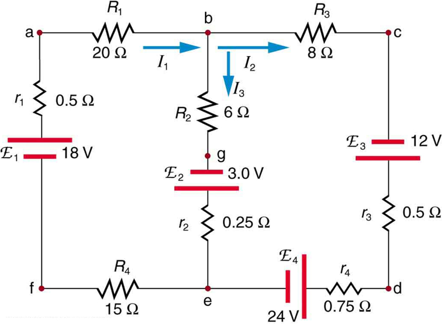
3: (a) What is the potential difference going from point a to point b in Figure 7? (b) What is the potential difference going from c to b? (c) From e to g? (d) From e to d?
4: Apply the loop rule to loop afedcba in Figure 7.
5: Apply the loop rule to loops abgefa and cbgedc in Figure 7.
Problem Exercises
1: Apply the loop rule to loop abcdefgha in Figure 5.
2: Apply the loop rule to loop aedcba in Figure 5.
3: Verify the second equation in Example 1 by substituting the values found for the currents [latex]\boldsymbol{I_1}[/latex] and [latex]\boldsymbol{I_2}[/latex].
4: Verify the third equation in Example 1 by substituting the values found for the currents [latex]\boldsymbol{I_1}[/latex] and [latex]\boldsymbol{I_3}[/latex].
5: Apply the junction rule at point a in Figure 8.
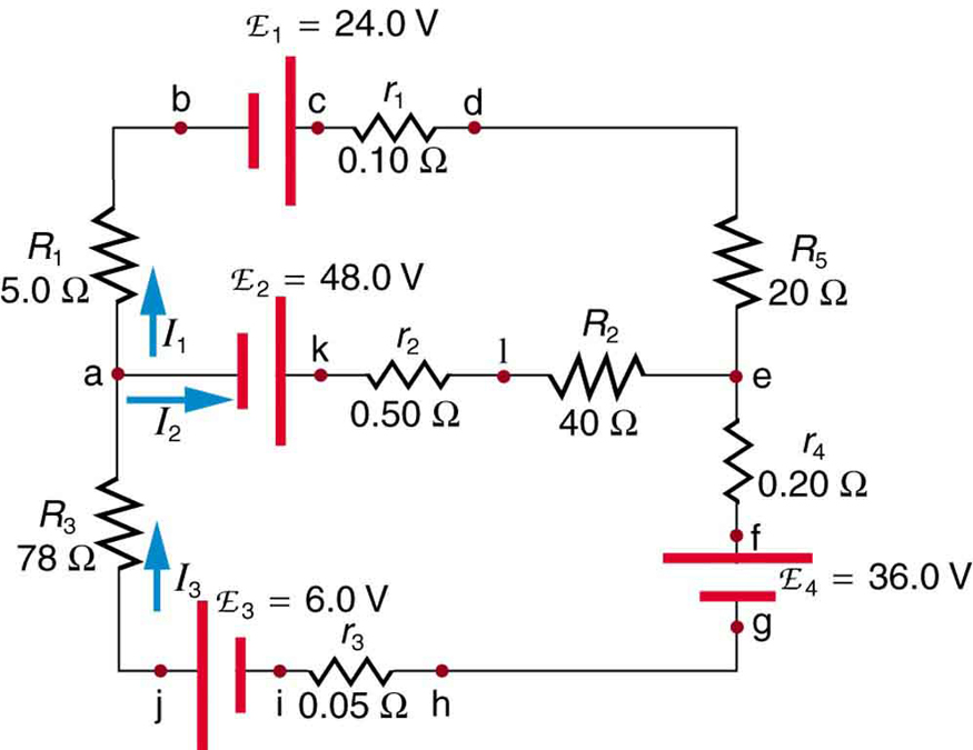
6: Apply the loop rule to loop abcdefghija in Figure 8.
7: Apply the loop rule to loop akledcba in Figure 8.
8: Find the currents flowing in the circuit in Figure 8. Explicitly show how you follow the steps in the Chapter 21.1 Problem-Solving Strategies for Series and Parallel Resistors.
9: Solve Example 1, but use loop abcdefgha instead of loop akledcba. Explicitly show how you follow the steps in the Chapter 21.1 Problem-Solving Strategies for Series and Parallel Resistors.
10: Find the currents flowing in the circuit in Figure 7.
11: Unreasonable Results
Consider the circuit in Figure 9, and suppose that the emfs are unknown and the currents are given to be [latex]\boldsymbol{I_1 = 5.00 \;\textbf{A}}[/latex], [latex]\boldsymbol{I_2 = 3.0 \;\textbf{A}}[/latex], and [latex]\boldsymbol{I_3 = -2.00 \;\textbf{A}}[/latex]. (a) Could you find the emfs? (b) What is wrong with the assumptions?
Glossary
- Kirchhoff’s rules
- a set of two rules, based on conservation of charge and energy, governing current and changes in potential in an electric circuit
- junction rule
- Kirchhoff’s first rule, which applies the conservation of charge to a junction; current is the flow of charge; thus, whatever charge flows into the junction must flow out; the rule can be stated [latex]\boldsymbol{I_1 = I_2 + I_3}[/latex]
- loop rule
- Kirchhoff’s second rule, which states that in a closed loop, whatever energy is supplied by emf must be transferred into other forms by devices in the loop, since there are no other ways in which energy can be transferred into or out of the circuit. Thus, the emf equals the sum of the [latex]\boldsymbol{IR}[/latex] (voltage) drops in the loop and can be stated: [latex]\boldsymbol{\textbf{emf} = Ir + IR_1 + IR_2}[/latex]
- conservation laws
- require that energy and charge be conserved in a system
Solutions
Check Your Understanding
1: Kirchhoff's rules can be applied to any circuit since they are applications to circuits of two conservation laws. Conservation laws are the most broadly applicable principles in physics. It is usually mathematically simpler to use the rules for series and parallel in simpler circuits so we emphasize Kirchhoff’s rules for use in more complicated situations. But the rules for series and parallel can be derived from Kirchhoff’s rules. Moreover, Kirchhoff’s rules can be expanded to devices other than resistors and emfs, such as capacitors, and are one of the basic analysis devices in circuit analysis.
Problem Exercises
9: (a) [latex]\boldsymbol{I_1 = 4.75 \;\textbf{A}}[/latex]
(b) [latex]\boldsymbol{I_2 = -3.5 \;\textbf{A}}[/latex]
(c) [latex]\boldsymbol{I_3 = 8.25 \;\textbf{A}}[/latex]
11: (a) No, you would get inconsistent equations to solve.
(b) [latex]\boldsymbol{I_1 \neq I_2 + I_3}[/latex]. The assumed currents violate the junction rule.
