Chapter 16 Oscillatory Motion and Waves
121 16.6 Uniform Circular Motion and Simple Harmonic Motion
Summary
- Compare simple harmonic motion with uniform circular motion.

There is an easy way to produce simple harmonic motion by using uniform circular motion. Figure 2 shows one way of using this method. A ball is attached to a uniformly rotating vertical turntable, and its shadow is projected on the floor as shown. The shadow undergoes simple harmonic motion. Hooke’s law usually describes uniform circular motions ([latex]\boldsymbol{\omega}[/latex]constant) rather than systems that have large visible displacements. So observing the projection of uniform circular motion, as in Figure 2, is often easier than observing a precise large-scale simple harmonic oscillator. If studied in sufficient depth, simple harmonic motion produced in this manner can give considerable insight into many aspects of oscillations and waves and is very useful mathematically. In our brief treatment, we shall indicate some of the major features of this relationship and how they might be useful.
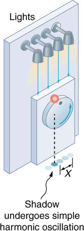
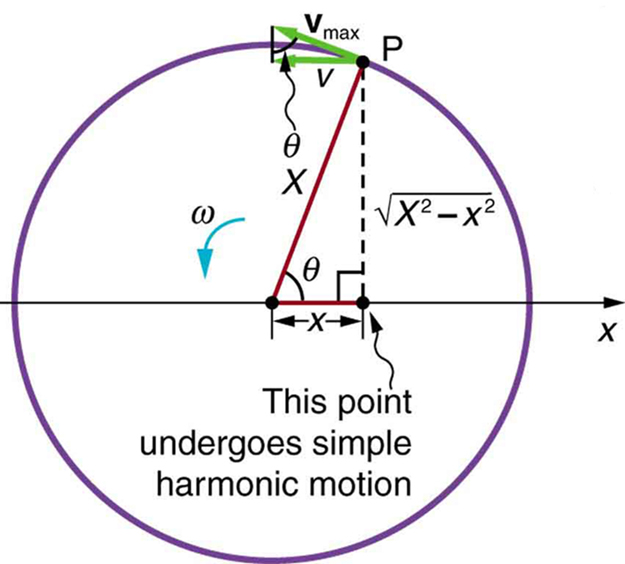
Figure 3 shows the basic relationship between uniform circular motion and simple harmonic motion. The point P travels around the circle at constant angular velocity[latex]\boldsymbol{\omega}.[/latex]The point P is analogous to an object on the merry-go-round. The projection of the position of P onto a fixed axis undergoes simple harmonic motion and is analogous to the shadow of the object. At the time shown in the figure, the projection has position[latex]\boldsymbol{x}[/latex]and moves to the left with velocity[latex]\boldsymbol{v}.[/latex]The velocity of the point P around the circle equals[latex]\boldsymbol{\bar{v}_{\textbf{max}}}.[/latex]The projection of[latex]\boldsymbol{\bar{v}_{\textbf{max}}}[/latex]on the[latex]\boldsymbol{x}[/latex]-axis is the velocity[latex]\boldsymbol{v}[/latex]of the simple harmonic motion along the[latex]\boldsymbol{x}[/latex]-axis.
To see that the projection undergoes simple harmonic motion, note that its position[latex]\boldsymbol{x}[/latex]is given by
where[latex]\boldsymbol{\theta=\omega{t}},\:\boldsymbol{\omega}[/latex]is the constant angular velocity, and[latex]\boldsymbol{X}[/latex]is the radius of the circular path. Thus,
The angular velocity[latex]\boldsymbol{\omega}[/latex]is in radians per unit time; in this case[latex]\boldsymbol{2\pi}[/latex]radians is the time for one revolution[latex]\boldsymbol{T}.[/latex]That is,[latex]\boldsymbol{\omega=2\pi/T}.[/latex]Substituting this expression for[latex]\boldsymbol{\omega},[/latex]we see that the position[latex]\boldsymbol{x}[/latex]is given by:
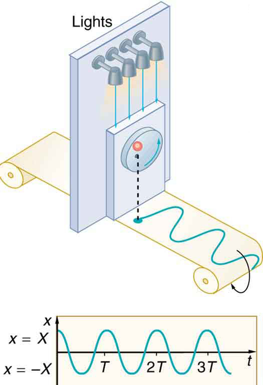
This expression is the same one we had for the position of a simple harmonic oscillator in Chapter 16.3 Simple Harmonic Motion: A Special Periodic Motion. If we make a graph of position versus time as in Figure 4, we see again the wavelike character (typical of simple harmonic motion) of the projection of uniform circular motion onto the[latex]\boldsymbol{x}[/latex]-axis.
Now let us use Figure 3 to do some further analysis of uniform circular motion as it relates to simple harmonic motion. The triangle formed by the velocities in the figure and the triangle formed by the displacements ([latex]\boldsymbol{X,\: x,}[/latex]and[latex]\boldsymbol{\sqrt{X^2-x^2}}[/latex]) are similar right triangles. Taking ratios of similar sides, we see that
We can solve this equation for the speed[latex]\boldsymbol{v}[/latex]or
This expression for the speed of a simple harmonic oscillator is exactly the same as the equation obtained from conservation of energy considerations in Chapter 16.5 Energy and the Simple Harmonic Oscillator.You can begin to see that it is possible to get all of the characteristics of simple harmonic motion from an analysis of the projection of uniform circular motion.
Finally, let us consider the period[latex]\boldsymbol{T}[/latex]of the motion of the projection. This period is the time it takes the point P to complete one revolution. That time is the circumference of the circle[latex]\boldsymbol{2\pi{X}}[/latex]divided by the velocity around the circle,[latex]\boldsymbol{v_{\textbf{max}}}.[/latex]Thus, the period[latex]\boldsymbol{T}[/latex]is
We know from conservation of energy considerations that
Solving this equation for[latex]\boldsymbol{X/v_{\textbf{max}}}[/latex]gives
Substituting this expression into the equation for[latex]\boldsymbol{T}[/latex]yields
Thus, the period of the motion is the same as for a simple harmonic oscillator. We have determined the period for any simple harmonic oscillator using the relationship between uniform circular motion and simple harmonic motion.
Some modules occasionally refer to the connection between uniform circular motion and simple harmonic motion. Moreover, if you carry your study of physics and its applications to greater depths, you will find this relationship useful. It can, for example, help to analyze how waves add when they are superimposed.
Check Your Understanding
1: Identify an object that undergoes uniform circular motion. Describe how you could trace the simple harmonic motion of this object as a wave.
Section Summary
A projection of uniform circular motion undergoes simple harmonic oscillation.
Problems & Exercises
1: (a)What is the maximum velocity of an 85.0-kg person bouncing on a bathroom scale having a force constant of[latex]\boldsymbol{1.50\times10^6\textbf{ N/m}},[/latex]if the amplitude of the bounce is 0.200 cm? (b)What is the maximum energy stored in the spring?
2: A novelty clock has a 0.0100-kg mass object bouncing on a spring that has a force constant of 1.25 N/m. What is the maximum velocity of the object if the object bounces 3.00 cm above and below its equilibrium position? (b) How many joules of kinetic energy does the object have at its maximum velocity?
3: At what positions is the speed of a simple harmonic oscillator half its maximum? That is, what values of[latex]\boldsymbol{x/X}[/latex]give[latex]\boldsymbol{v=\pm{v}_{\textbf{max}}/2},[/latex]where[latex]\boldsymbol{X}[/latex]is the amplitude of the motion?
4: A ladybug sits 12.0 cm from the center of a Beatles music album spinning at 33.33 rpm. What is the maximum velocity of its shadow on the wall behind the turntable, if illuminated parallel to the record by the parallel rays of the setting Sun?
Solutions
Check Your Understanding
1: A record player undergoes uniform circular motion. You could attach dowel rod to one point on the outside edge of the turntable and attach a pen to the other end of the dowel. As the record player turns, the pen will move. You can drag a long piece of paper under the pen, capturing its motion as a wave.
Problems & Exercises
1:
a). 0.266 m/s
b). 3.00 J
3:
[latex]\boldsymbol{\pm\frac{\sqrt{3}}{2}}[/latex]
