Introduction

In this section we’ll look at a type of PCR that allows you to assess the level of expression of a gene in a variety of contexts. Here are two sample questions that could be answered using qPCR (quantitative PCR).

i. Is the gene differently expressed in different tissues or stages during development? Or is it expressed throughout the organism at all times?

ii. Is this gene expressed more or less in tumour cells compared to non-cancerous tissue in the same individual?

There are other types of questions that can be answered as well, such as whether a particular drug treatment or other factor (exposure to high temperature or certain types of stress) can alter gene expression or whether individuals with different health concerns tend to have certain genes expressed more or less than in individuals that don’t have that health condition. We’ll stick with just the two questions listed above for this section, but keep in mind that there are others that can be addressed.

The key to qPCR is that the reaction is monitored as it is running, and the amplification process itself can tell us what the relative amount of template was in the original sample. As you can probably guess, in this type of PCR controls are extremely important.

Click here for the powerpoint slides presented in the video below.

We will also briefly touch on RNA-Seq, which is an approach that leads to sequencing of all RNAs in a sample, through first reverse transcribing all the RNAs in the sample and then doing high throughput (large scale) sequencing of the cDNAs to get a sense of not only which genes are expressed in the sample but how much they are expressed. Because Next Generation sequencing is used for this, it is possible to sequence multiple samples in the same flow cell.

A. Review of PCR Amplification:

A-1. How it works

In order to understand how real-time, quantitative PCR works, we have to review how PCR amplification proceeds normally. You may wish to review the PCR worksheet from earlier in the semester. In it, you were asked to follow the first few amplifications of a PCR reaction. In those first few cycles, some linear products were made (that amplified by adding the same number of strands each cycle) and the intended product was made by very slightly more than doubling it each cycle. In our theoretical example, at the end of the PCR, we had well over a billion pieces of the intended product (the exponential amplification) and 60 strands each of the linear products. This shows the enormous difference between linear and exponential amplification. By the time we are into the 4th or 5th cycle in our theoretical example, the linear pieces are insignificant in number and they can be ignored. We can consider that the product is doubling in amount each cycle and that is accurate enough.

But the product doesn’t double indefinitely! At some point, the primers and nucleotides begin to decline in amount; they get used up. And without these, we cannot build any more new DNA strands. And even though the enzyme is thermo-tolerant, and we could cycle it to 95^oC and back 30 or more times, eventually the enzyme will begin to lose its activity. So if we were to observe the amplification process- by measuring the amount of product each cycle, we would see a sigmoidal curve. It takes a few cycles to get going, then there is the rapid exponential amplification, but the curve begins to tail off at the top. The curve below comes from BioRad. They sell qPCR reagents and the companies who sell the reagents for a technique can be a valuable source of information for how the technique works, and how to troubleshoot it. If you want to know the drawbacks of a particular approach you can sometimes find this out from the company too but may have to look elsewhere for this information. In the curve you will see an almost flat “initiation” phase at the beginning of the PCR, and then the exponential phase in the middle- where the slope is steepest, followed by the “plateau” phase near then end.

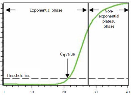
In standard PCR we don’t think much about this curve unless the reaction fails and we are having to troubleshoot. But in qPCR all the focus really is on this curve and the cycle at which our reaction crosses out of the initiation part and into the steep exponential phase.

A-2. What it is used for

In  regular PCR we are usually aimed at amplifying a particular product. We don’t monitor the course of the amplification because our goal is to run a bit of the reaction on a gel at the end of the process to see if we have the correct product. Then we purify the product using a column prep. Usually we want to clone the DNA or sequence it, or digest it. There is some downstream use for it that we have in mind. So our focus is just on getting the product.

For qPCR, (quantitative PCR) as the name suggests, we are using the PCR reaction itself to measure something – namely the amount of template we began with. The amount of template started with is used as a measure of something we want to know about – copy number of a DNA sequence, viral load, or expression of a gene. This will be described in the next section.

Click here for the powerpoint slides presented in the video below.

B. qPCR:

B-1. What it is used for

Note that I provided some of this information in the introductory part of the lecture above and am just providing a few more details here.

qPCR is a method to measure the amount of template a PCR reaction started with. If the experiment is carefully designed and quantified, the amount of template can indicate the following:

B1-i. Copy number

In the genomes of many organisms there are certain genes that exist with copy number variants (CNVs). This means that some individuals have up to 4 (perhaps more) copies of the gene and others have just one. This occurs through gene duplication and/or deletion. The genes involved are obviously ones where having more or fewer copies is not lethal, but the different copy numbers could be associated with specific health conditions. Sometimes the duplications and deletions are long sequences that include more than one gene plus all the sequence between the genes.

B1-ii. Gene expression

A very common use of qPCR is the measurement of different levels of gene expression in particular stages of an organism, different cell cultures subjected to certain treatments, or diseased and non-diseased tissues of the same individual. In the last case, tumour and non-tumour tissue from the same patient can be assessed. If we find genes that are expressed at higher levels in a tumour we may be able to identify therapeutic targets that are most likely to work for this individual patient. Genes that are less expressed in the tumour might also suggest a treatment- perhaps if the cells were exposed to more of that particular gene product it would inhibit the growth of the tumour. This is one of the technologies that is taking us toward personalized medicine, the ability to tailor prevention strategies and treatments to a particular individual’s unique traits.

B1-iii. Viral load

When a person, animal or plant is infected with a virus, we want to identify which virus they have. We can use regular PCR to do a diagnostic amplification. We use primers specific to a certain virus and we use the presence or absence of the expected product to answer a yes/no question: does the sample have this virus or not? What we cannot usually tell from standard PCR is how much virus the sample has. Suppose we are treating the individual with medications and we want to know if the treatment has been effective. In that case we might be able to detect the virus in the pretreatment and post treatment samples through standard PCR but we couldn’t tell if the treatment had reduced the amount of virus. qPCR can help us quantify the amount of virus (or bacteria, or other pathogen) in a sample. This allows us to determine how effective a treatment has been and perhaps to make changes to the treatment strategy.

There are lots of other applications but these are enough to start with.

B-2. How qPCR works:

B2-i.  The key: incorporation of fluorescence

The key to qPCR is the use of SYBR green or other fluorescent dyes that specifically bind double-stranded DNA (dsDNA). These do not fluoresce (or have a low level of background fluorescence) until they are bound to dsDNA. So as a PCR reaction proceeds, the amount of fluorescence increases as the number of double stranded DNA molecules increases. The output of the fluorescence is measured; it indicates the amount of product in the tube at any particular time.

The qPCR machines have a setup that shines light on each of the wells as the reaction proceeds. The SYBR green or other dyes are excited by the light (497 nm, in the blue range) and then the light they emit in response is detected and the information is fed into a computer program. Near the beginning of the reaction there is not a lot of fluorescence and the fluorescent signal is weak and variable. We say that there is a lot of “noise”. As we begin to enter the exponential phase, the signal is strong and reliably related to the number of ds-DNA molecules in the reaction.

Click here for the powerpoint slides presented in the video below.

B2-ii. Ct values

CT stands for “crossed threshold” and it is a point at which the amplification passed a specific point, and where the doubling rate can tell the you relative template amount.  The initial steps of the PCR are a bit chaotic when plotted and comparing samples before the exponential phase is not reliable. Similarly, different reactions begin to plateau at different points and with similar (usually) final amounts of product and it is not useful to compare samples at this point either. You need to be able to compare the samples during the early exponential phase. At this point, you have enough product for the doubling times to be very consistent and the comparisons we want to make are meaningful during this stage. We are nowhere near running out of primers or nucleotides at this point, for instance, whereas nearer the upper part of the exponential phase this may be starting to happen.  Watch the videos to understand the relationship between your amount of starting material and the Ct value.  If you start with twice as much of the template in an experimental tube than the control, the threshold should be crossed in the experimental sample one cycle (one doubling) sooner than the control. If you start half as much relative to the control, it should take one extra cycle (one doubling) to reach the threshold amount of product.

The computer program will provide traces of the amplifications and a trace that plots the log of the fluorescence again the cycles.  You will see a lot of noise at the bottom of the graph before the sample moves into robust exponential amplification. And this allows you to select the appropriate threshold level. You want to choose a level that is well above the noise of the signal, but not too close to the plateau.

You would have amplified a series of diluted standards that can be used to then produce a reference plot of the Ct value against the log of the copy number of the DNA. You need to have very accurately quantified DNA samples for this so that you know exactly how much template was added to each of the standard tubes. This is one of the most important controls and should produce a straight line. If it does not, you may need to redo the experiment. If you have a nice straight line, you can interpolate the Ct value for your sample and find the log of the amount of template you had in your sample. This is how you can determine the absolute amount of template from a particular sample. You ought to have run replicates of your experimental samples as well and these should yield a similar value. If you have done a dilution series of your experimental samples, all should give consistent results. For instance if you ran a couple of experimental samples, these should give close to the same amount of starting material. And if you ran a couple of 1/10 dilutions of the experimental template, these should also agree with each other and when you use the graph to figure out the amount of template in the dilutions it should be 1/10 of what the experimental sample was.  Otherwise there has been inconsistent pipetting and the results won’t be reliable.

Click here for the powerpoint slides presented in the video below.

Note that you don’t necessarily have to figure out the exact absolute amount of your template; depending on what research question you are asking, you can also opt to make a relative comparison. An example could be to test a mutant strain of a plant or animal and determine how much of a particular gene or genes are expressed in the mutant relative to wild type. The recording below has a couple of real examples from the SFU BISC and MBB departments.

Click here for the powerpoint slides presented in the video below.

C. Controls:

C-1. Enhancing consistency in the results

Careful design of the experiment is essential to success. You isolate the RNA of the different samples you want to test and make cDNA with the mRNAs. Or in some experiments you isolate genomic DNA to use as a template (when assaying copy number for instance). If you are trying to compare the amount of template in different samples it is important to carefully quantify the cDNA or genomic DNA you are using. If we are trying to get at just a 4 fold difference in copy number between two samples, accidentally adding more starting material of one over the other could either exaggerate the difference between them or minimize it. You might still be able to interpret the results through a comparative analysis but it is more work.

Consistency is also important. It is useful to set up replicates of your experimental samples. You might do several dilutions of each experimental sample and then perform 2 or 3 replicates of each of these dilutions. You expect to get very similar results with each replicate of the same sample and the results from the dilutions should all be consistent with each other. This is described above, but it is worth emphasizing. A lot of the techniques we use depend on proper controls for consistency and reliability. Understanding the purpose of the controls is essential.

The use of mastermixes for the reagents common to all of the samples will help to reduce variation between samples due to pipetting inaccuracies. For most experiments the first mastermix would include: buffer, nucleotides and enzyme and some water. These will be common to every sample. The amounts used are increased by about 10% to account for possible pipetting inaccuracies. The mastermix is thoroughly mixed to ensure equal distribution of all the substances and then aliquoted into sub-master mixes. In these tubes the next reagents are added, usually the primers because in the experiment you are assaying different genes, even if only for the controls. Finally the sub-master mix reactions are aliquoted into PCR tubes and the final reagent is added: the template for each reaction.

Staying organized is really important because you often have replicates of a particular experimental sample as well as a dilution series of one or more of the genes and you have to put each tube into the machine at a prescribed location. Because the experiments are fairly large scale, you have to be super careful not to mix up the tubes or the labeling of the tubes. The computer software helps you stay organized by mapping out in advance which sample will be in each well of the thermocycler.

C-2. “Housekeeping” genes as a reference

As has been mentioned in the recorded lectures, housekeeping genes are often used as references in qPCR experiments. These are genes that are relatively consistently expressed from one cell type to another and so we often measure the expression of our experimental genes in comparison to these reference genes. Common housekeeping genes include enzymes like glyceraldehyde-3-phosphate dehydrogenase and phosphoglycerate kinase; these both act in glycolysis which is how cells produce energy. Actin and tubulin are proteins that are part of the cytoskeleton of all cells and ribosomal proteins are also found in all cells at very high levels. Ubiquitin is also used. You can maybe tell from the name that it is found in all cell types.

Most experiments include the use of two housekeeping genes as references. Some may include more. The results of the qPCR should show consistency for all the housekeeping genes used.  If a gene is expressed 5X more than housekeeping gene A in one sample and 10X more than housekeeping gene B in the same sample, it would not make sense for that gene to be expressed the same as housekeeping gene A in the second sample but 5X less than housekeeping gene B in that sample.  If we saw results like that we would have to question either our sample preparation or whether the housekeeping genes are really expressed consistently from one sample to another. Thus it is important to do controls to ensure that the housekeeping genes indeed are expressed consistently in the different tissues or samples you are testing, because even these genes may vary somewhat between samples.

D. RNA-seq – A different way to get at differential gene expression:

The name RNA-Seq is misleading because it sounds like we can directly sequence the RNA which is not correct. It has to be reverse transcribed into cDNA first and then sequenced. The process of RNA -Seq is very similar to Next Gen sequencing, so I will just talk a bit about sample preparation and a bit about the collection of the data.

We begin by isolating just mRNA by targeting the polyA tail. Magnetic beads coated with oligo dT would be a good choice for this step.  There is another approach involving an enzyme that degrades the ribosomal RNA but this still leaves tRNA. So I think the best approach is the dT approach. This is of course just an opinion – I have not personally done this technique. This is followed by breaking the RNA into small pieces similar to what is done in the DNA preparation for Next Generation sequencing. Then the RNA is reverse transcribed to make double stranded DNA. Random primers must be used for the first strand synthesis, since most of the pieces will lack the polyA tail. The second strand is made with DNA polymerase.  The molecules are from that point on treated exactly like the DNA pieces for Next Generation sequencing; they are polished, adaptors are added and they are PCRd a few times to get amplification of the DNA and to make it complementary throughout. The PCR amplifications are kept fairly low to minimize the chances of errors being incorporated into the sequences.

Cluster formation and actual sequencing proceeds as described in Chapter 10. Single end or paired end sequencing can be done according to preference.  Cost seems to be a main factor; paired end sequencing is somewhat more expensive. Before the cluster formation and sequencing are done, there are multiple quality control measures that are taken. These include checking that the DNA pieces are on average the expected length and confirming the concentration of the DNA in the sample. If we are trying to compare two samples, such as tumour and non-tumour tissue from the same patient and our aim is to identify which genes are expressed more and less in the tumour tissue compared to the normal tissue, then we need a similar concentration of cDNA pieces so that the comparison is easier to make. If we added 5X more cDNA from the tumour tissue to the flow cell compared to cDNA from the non-tumour tissue, it would take more work trying to identify genes that were really over-expressed in the tumour sample.

Once the sequencing is complete the data are analyzed. Prior to that, some reads have to be eliminated from the data set. Sometimes a certain cluster has a very poor signal or a signal that cannot be interpreted by the computer. This could be due to mistakes in incorporation of the fluorescent terminator in some strands or failure to cleave the fluorophore or blocking group in others.  These strands will be out of sequence with the others in the cluster and so the signal gets “messy”.  Sometimes two clusters overlap with each other and their individual results cannot be separated. These have to be ignored. Sometimes there are also artifacts- sometimes two adaptors manage to ligate to each other without a DNA piece between them. These reads must be eliminated. And the adaptor sequence is trimmed out of the reads as well.

Then the DNA sequences are matched to the genomic sequence.  The number of reads for each gene can be determined. “Reads per gene” means the number of fragments of DNA that were sequenced that correspond to each particular gene.  We expect that highly expressed genes will be represented more in a particular sample than non-expressed genes or genes expressed at lower levels.

The data need to be normalized and there are different ways to do this. The simplest way is to determine how many total “reads” there were for each of your samples and adjust the data to reflect that. When you do the gene expression lab next week (following up on the mRNA samples you collected near the beginning of the semester) you will go through a small amount of data to practice interpretation of it.

Here is a link to a StatQuest video in which a guy with a pretty deadpan voice and a sense of humour explains how RNA-Seq works. It is quite oversimplified in the “sequencing” part, but the rest is potentially of value.

RESOURCES

Here is a link to a company (in the lower mainland!) webinar that explains how to do RNA-Seq. I was quite impressed to see a former SFU student hosting the webinar! I can remember he took some courses with me which I sincerely hope helped him along his path- you never really know what kind of effect you have (or not) on people in the long term.  This webinar is a bit long – but there is good information here.

Previous (Chapter 11)Next (Chapter 13)