Introduction

This short chapter will take you through the early DNA sequencing done by the Sanger method (though with a nod to the Maxam-Gilbert method), and then we’ll look at some of the improvements to the method. Some sequencing is still done this way so it may be useful if you go on in Molecular Biology. But even when the technique is not used any more it will be helpful to understand how it works – because chain termination (the principle behind Sanger sequencing) is used in other, more modern, methods as well.

DNA sequencing is done for several reasons. Perhaps a large number of DNAs have been PCR amplified from soil or water, and you wish to identify what type of organisms are found in the sample and how their genes are related to those of other organisms. You may be making cDNAs from certain tissues, or even from a tumour and the normal non-tumour tissue from the same individual in order to figure out what the gene expression differences are between the cancer cells and the normal cells. In cases like this you don’t know which genes you’ve sampled and you perform DNA sequencing to find out. In other cases you’ve perhaps cloned a gene or several genes and before you proceed with additional work, you must confirm that the DNA is indeed the gene you think it is and that no errors were incorporated during the PCR. Sequencing is done for this reason also.

A. Two types of sequencing – Maxam-Gilbert, and Sanger methods:

In the 1980s there were two main methods for sequencing DNA: the Maxam-Gilbert method of differential cleavage and the Sanger chain termination method. The principle of the Maxam-Gilbert method was to isolate large amounts of DNA, label it and then cleave subsets of the sample at the different nucleotides. If the cut pieces were run on a gel, you could then infer the position of each nucleotide by the resulting size of the band on the gel.  The chain termination method involved synthesizing DNA in four separate reactions each of which had a small amount of a modified nucleotide that would not allow synthesis to proceed. As with the differential cleavage method, the resulting pieces were run on a gel and the sizes of the bands in each lane indicated the position of each nucleotide. Details of the procedures are given below. Both methods were used for some years; my boyfriend in grad school sequenced several genes via the Maxam-Gilbert method for his PhD project. However, over time the Sanger method became the method of choice for most sequencing.

A-1. Differential cleavage: Maxam-Gilbert Method (developed ~ 1976/1977)

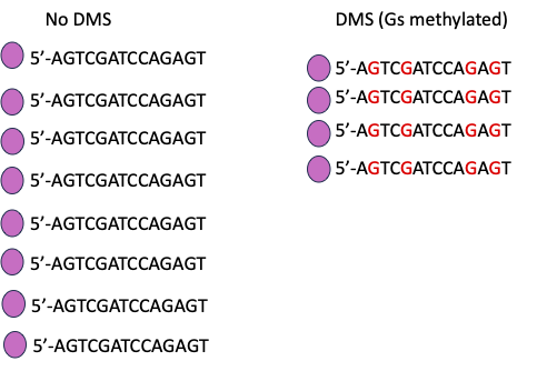
This is a very interesting sequencing method which was at first favoured over Sanger sequencing due to convenience.  It involved “end-labeling” the piece of DNA to be sequenced with a radioactive nucleotide.  Then the DNA was divided into 4 treatments, one for each nucleotide. There were two tubes for “purines”, A or G. In the first tube nothing was added and in the second dimethyl sulfate was added. This added a methyl group to the G nucleotides on the DNA.  Then both tubes were treated with formic acid to depurinate the DNA (remove the purine bases).  In the first tube both A and G would be cleaved (by a treatment with piperidine, see below), but in the second, only A was cleaved because the G had been protected by methylation.

The image below shows a short sequence (multiple copies; many copies were needed for best results) with an end label indicated by the pink blob at the 5′ ends of the molecules. In the DMS treated sample, the methylated (protected) Gs are shown in red.

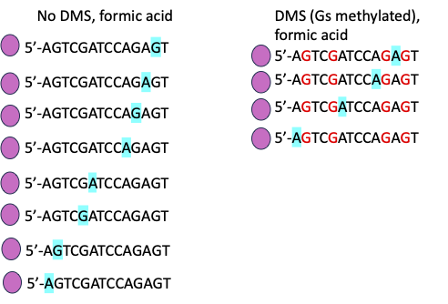
This image (below) indicates with blue highlight which bases will be removed by the acid treatment.

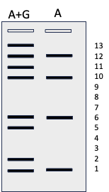
This image shows the lengths of fragments after cleavage (see below). It is slightly misleading because I’ve left in the nucleotides that were cleaved, just to indicate that each fragment shows the position of A and/or G. In reality, each piece would be one nucleotide shorter than I’ve shown it. Beside  that is the gel image we would see for this very small piece of DNA after the purine treatment. You can figure out where the A and G residues are on the sequence but not what the other nucleotides are. You need all four reactions to work in order to determine the complete sequence.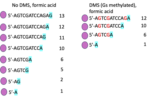

Two tubes for “pyrimidines” were also set up. In the first, nothing was added but in the second some sodium chloride was added which had the effect of protecting the C nucleotides from the treatment that modified the pyrimidines. Then both tubes were treated with hydrazine. In the first tube, both C and T nucleotides were altered but in the second only the Ts were altered. Study tip: make diagrams like the ones I made above, using the same sequence, but highlighting the pyrimidine treatments. Then make a picture of the gel with all four lanes shown and demonstrate that you can read the gel from bottom to top and get the complete sequence.  This is the best way to be sure you understand how this method works.

Finally all four tubes were treated with hot piperidine, which cleaves all modified bases. The reaction is done so that on average only one cleavage occurs per strand of DNA. This means that each tube is filled with strands of DNA that are cut once to produce a smaller, labeled fragment. There are many fragments of all sizes in each tube.  The size of each piece tells you which nucleotide was in that position. The first tube shows the sizes of molecules cut at A and G while the second tube shows only A. Therefore molecules in the first lane but not the second indicate G while molecules in both lanes indicate A.  The third tube shows the sizes of the molecules that end with C and T while the fourth shows only those that end with T. Therefore the molecules in the first but not second lane are the molecules ending with C and the ones in both lanes are the molecules that end with T. It is not as complicated as it sounds and for several years it was the preferred sequencing method.

However, once the Sanger sequencing underwent some improvements, it soon eclipsed the Maxam-Gilbert method. 

A-2. Chain termination: Sanger method

The Sanger method involves inferring the sequence of a DNA strand through synthesis. Fred Sanger, the developer of the method is one of very few people who have received two Nobel Prizes. One was  in Chemistry for his work on protein structure, in particular the structure of insulin, and the second was shared with Walter Maxam for their DNA sequencing methods.

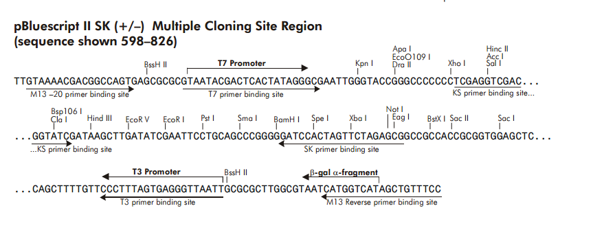
If you look at the polylinker of many plasmids, there are sites to either side of it that are designed for sequencing.  The image below shows the polylinker of the pBluescript plasmid. There are multiple primer sites shown in the image. On the left side of the polylinker, there are primers named (from the far left inwards) M13 forward, T7, and KS and on the right side are (from the far right inwards) M13 reverse, T3, and SK.  These are commercially available primers that can be purchased very inexpensively if you are doing your own sequencing.  Even more inexpensively, you can send your DNA from a plasmid prep to one of several companies that will sequence it for you using whichever of these standard primers you specify. You can also include your own custom designed primer in the tube with your DNA if need be.

This video is the introduction part of the Sanger sequencing lecture (click here for powerpoint slides):

A2-i. How the method works

Let’s look at how the method works. In Sanger sequencing, we prepare our DNA and then use one primer to synthesize one strand of it. We use a trick that causes the strands to end at random positions and  the size of each randomly terminated piece will indicate where the corresponding nucleotide was in the sequence.

The method uses dideoxynucleotides (ddNTPs). These have no 3′ OH and so no new nucleotides can be added to them. We call these terminators – because as the DNA strand is being synthesized, whenever a ddNTP is incorporated, that strand stops growing.

What do we need to do this type of sequencing? We need a single stranded template DNA – this the DNA we will sequence. We can obtain this fairly easily through denaturation of the plasmid  (or other DNA) we are using. It also requires a primer; DNA synthesis always needs a primer. And it needs a DNA polymerase. We used to mostly use Klenow for sequencing but we can also use Taq (which will be described more below). We also use nucleotides, dNTPs to build the new DNA strand. And we include a small proportion of ddNTPs. Initially there were 4 separate tubes to sequence one DNA template. In each tube all four dNTPs were added, and then one tube had a small amount of ddATP added to it. This is the A tube. Then another had a small amount of ddCTP added to it. This is the C tube. And so on. As DNA synthesis proceeds in the A tube, many DNA molecules are being made. Every time the enzyme finds a T in the template it will incorporate an A nucleotide in the DNA it is synthesizing. Occasionally that nucleotide will be a ddATP. This stops further synthesis of that strand. At the end of the sequencing there will be many molecules all of which end with an A. And many copies of the DNA strands of each size.

The same is true for the other tubes, each will have a set of DNA molecules that are all different sizes and each stops at a C in the C tube, and a G in the G tube and a T in the T tube. We then run these reactions on a polyacrylamide gel, which is able to resolve DNA molecules that differ in length by only one nucleotide.  The DNA bands at the bottom of the gel are the smallest and we can read the bands from the bottom of the gel up to determine the sequence.

Here is video to part of my lecture on the topic that explains this (click here for powerpoint slides):

B. Improvements to Sanger sequencing:

We are always improving on our techniques and one problem with Sanger sequencing was the large amount of template needed to do the synthesis reactions. The amount of product could sometimes be low, because we used Klenow enzyme. We had to work with isotopes which require extremely careful procedures. And we did 4 separate reactions to sequence one template DNA. So if one of those reactions failed, we could not determine the sequence. (This was true of the Maxam-Gilbert method also).  Modifications that improved Sanger sequencing include: the use of Taq polymerase and cycles of denaturation and synthesis, and the use of fluorescent terminators to detect the product pieces.

B-1. Cycle sequencing

If we synthesize DNA in our sequencing reaction by doing “cycle” sequencing using Taq polymerase, we can get a much larger amount of product. There are many more pieces made of each product strand and so these show up better on the gel.  When we first began to do this we were still dealing with the health and safety concerns of working with isotopes. This meant we had to shield the thermocycler and do careful swipe testing after using it. Swipe testing is a way to monitor whether equipment or working spaces are contaminated with radioactivity. If they were contaminated that was a serious issue and an arduous clean up/decontamination process took place.

B-2. Fluorescent terminators

To eliminate the safety concerns of working with isotopes we turned to fluorescence. We used differently labeled  ddNTPs for each reaction.  The the ddATP would be labeled with red fluorescence, while the ddCTP might be labeled with yellow fluorescence. So each strand of DNA that was synthesized in the sequencing reaction would end with a ddNTP and a unique, nucleotide specific fluorescent label. This meant that the reaction could all be done in a single tube because we could identify which nucleotide was at each position by the colour of the fluorescence. So not only is the work safer but it is more efficient as well.

To detect the fluorescence a computer apparatus is set up. Each reaction is run in a polyacrylamide gel in a single lane and towards the end of the gel, there is a laser that excites the fluorescence and a photomultiplier that detects the light emitted and sends the information to the computer for analysis. Each molecule is “read” as it passes the detector and the colour is recorded. This computer  produces a trace, showing the fluorescence detected in peaks, where each peak corresponds to a nucleotide.

Click here for powerpoint slides presented in the video below.

B-3. Scaling the process up

Currently the companies that do Sanger sequencing use a partly automated system. It involved doing the reactions – up to 384 of them – in a capillary plate. Each reaction represents one template so many can be done simultaneously.  The gels are not traditional gels any more- very narrow capillary tubes are filled with polyacrylamide and one end is set into each well of the capillary plate – which is the “cathode” plate, acting as the negative pole in the electrophoresis. A current is set up and the DNA moves from the wells of the plate through the tiny capillary tubes toward the anode. The DNA bands are read as they pass by the laser in quite the same way as previously described except on a much larger scale.

Click here for powerpoint slide presented in the video below.

C. Cloning Large Inserts:

C-1. Sequences of 1-10 kb: Primer walking

When Sanger sequencing is working very well we can expect usually around 600 to 800 bases of sequence from each run though sometimes we can get a bit more. But there is a limit to the enzyme’s activity and the amount of terminator that you can use. If you use too little you get too few pieces of each size so the signal is too weak. If you use too much (proportionately) this will favour smaller pieces as the chance of incorporation will increase.  The limit seems to be maybe 1000 bases of sequence.

Suppose then that you have an insert that is 1 kb in length? That works very well. We sequence in two reactions, one from either side of the insert and we get quite a bit of overlap in the middle part of the sequence. We like to get coverage from both directions. Sometimes there are issues with certain sequences- I mentioned compressions previously, in the recording about running and reading the gel. In this case a segment with multiple Gs sometimes produced bands that squish together so it can be difficult to tell if for instance there are 3 Gs or 4.  However, strangely, when we sequence from the other side the Cs don’t do that so we can compare the trace with the Cs to the trace with the Gs and the Cs will show us the correct number of Gs as well. All methods have some kind of idiosyncrasy that we have to work around. For sequence to be published in a data base, you want to have sequenced the same sequence multiple times in both directions. For the human genome, the high quality sequence has 11-fold coverage from each side of the sequence from 5 individuals (that is the DNA from the five individuals are each covered 11 times in each direction – at least that is how I read it). This gives us confidence in the accuracy of the DNA sequence.

Suppose you have an insert that is 6 kb.   The best sequencing from each end gives you only 1/3 of the sequence and coverage in only one direction. So we have to use the sequencing data we get from the first “read” to design a primer to sequence the next section of the insert. And so on. It is slow because we have to order the primers and wait for them to arrive before doing the next sequencing reaction. That is why it is called “primer walking”; it is a slow process, done step-by-step.

If we have cloned a well-known gene we can take the shortcut of ordering primers that we anticipate will be well spaced across the gene and use these to do a bunch of sequencing reactions simultaneously. Then we can put together all the sequence data at once to see what the full sequence of the insert is. We space the primers out so that each sequence we generate will overlap with the next one, and we design both forward and reverse primers for separate sequences in each direction. It is essential to know the gene you are dealing with and the sequence of it with some certainty or the results of the shortcut could be disappointing.

C-2. Sequences of more than 50 kb: Shotgun sequencing

We don’t want to do primer walking if we are trying to sequence a huge insert (for instance if we cloned DNA into a viral vector or an artificial chromosome). It would take much too long to walk across 100 kb of sequence about 600 bases at a time. Instead we use a method called shotgun sequencing. The name comes from the fact that shotgun shells are full of lead pellets and they spray out to increase the chances that some will hit the target. In shotgun sequencing you extract the DNA and cut it into smaller, but overlapping (this is critical) pieces. Each small piece is cloned into a separate vector and a library is produced. A library is a collection of clones containing a large number of pieces of DNA from a single sample. It could be all the expressed sequences (cDNAs) in a certain tissue, all the DNA in the genome of an organism, or all the genomes of multiple organisms in a soil or water sample.  In this example, though, we are just talking about a single piece of DNA that is maybe 50 kb or larger.

The vectors are transformed into bacteria that are selectively plated on antibiotic plates like described in Chapter 6 except on a much larger scale and every colony is likely to have a different DNA insert. The colonies are individually selected, grown up in liquid culture and plasmid preps are made. Each insert is sequenced. The pieces are all random and at first you don’t know how one sequence relates to another, but through computer assembly, finding overlaps between DNA sequences, you can put together “contigs”. These are contiguous sequences – that are beside each other in the original piece of DNA you wanted to sequence. A lot of sequencing reactions lead to a lot of overlap between the sequences and so we can be very sure of the contig we generate from our insert if we have 5 fold coverage or more. The sequencing doesn’t have to cover the entire insert either- since the DNA is broken randomly, if we do enough sequences we will have good coverage even if we only sequence the first few hundred nucleotides of the insert.  This is where automated sequencing and the use of biocomputing is essential. In the next chapter we are going to look at a way that we can do massive parallel processing, which refers to the ability to sequence millions of small fragments all at once. It relies on some of the principles in this chapter which you need to understand. Next week we are doing Next Gen sequencing on ancient DNA which I hope you will find interesting.

Click here for powerpoint slides presented in the video below.

Previous (Chapter 9)Next (Chapter 11)