19 PID controller
The PID controllers are widely used to improve the performance of closed-loop feedback systems. The integrator of a PID controller can capture the history of the system and its differentiator anticipates the future behavior of the system.
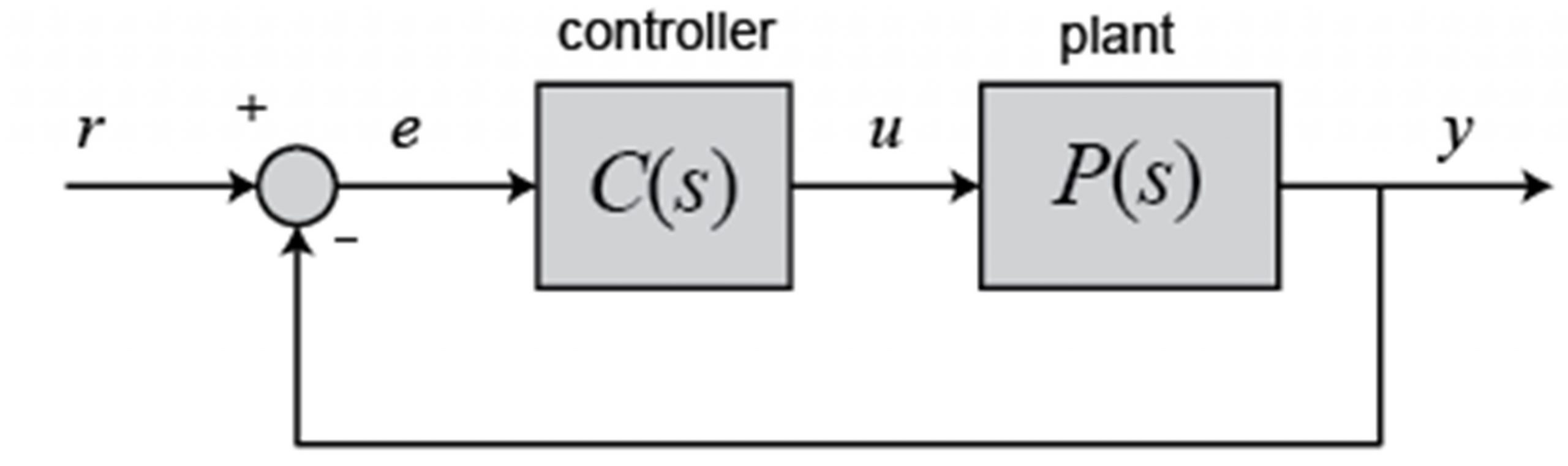
Considering a PID controller in a unity-feedback system such as the one shown in Figure 10.1, the input applied to the plant is obtained as:
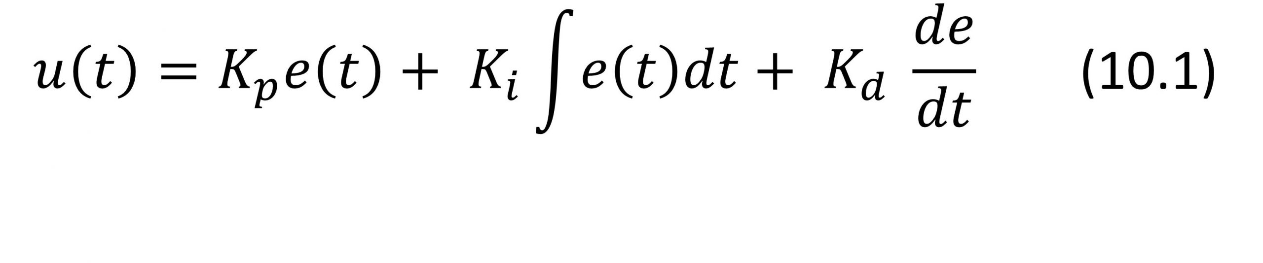
Where Kp is the proportional gain, Ki is the integral gain, and Kd is the derivative gain. Signal denotes the tracking error which is basically the difference between the desired output (reference) r, and the actual output y.
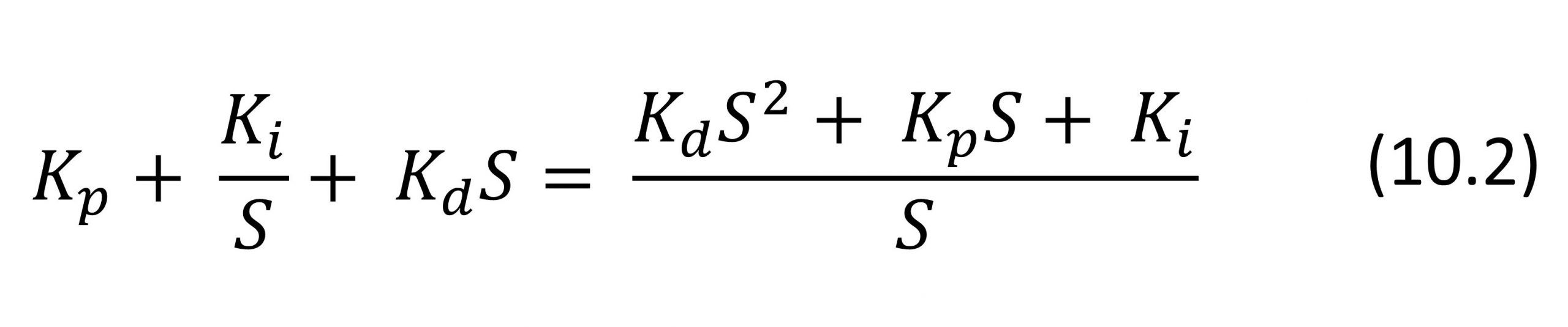
The transfer function of the PID controller is obtained by taking the Laplace Transform of (10.1).
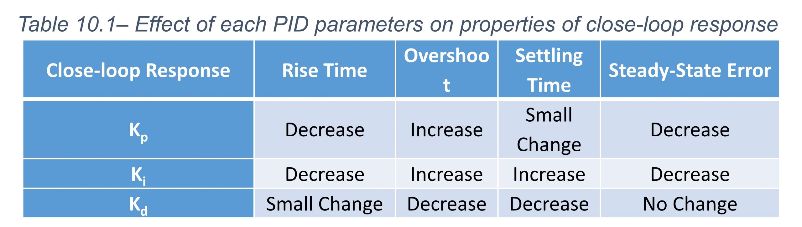
Increasing the proportional gain Kp increases the control signal for the same level of error and causes the controller to push harder and react faster which may result in higher overshoot. Increasing Kp also reduces the steady-state error.
The derivative term Kd in the controller allows the controller to “anticipate” the error. In other words, if the error begins sloping upward, the control signal u(t) will be increased. Note that the derivative term has no impact on the steady-state error.
The integral term Ki reduces the steady-state error. However, it is possible that the system becomes oscillatory.
Table 10.1 summarizes the general effects of each PID controller term (Kp, Kd, Ki) on a feedback system.
For designing a PID controller consider the following steps:
- Evaluate the open-loop response of the system to see what needs to be improved.
- Improve the rise time by adding a proportional control.
- Reduce the overshoot by adding a derivative control.
- Reduce the steady-state error by adding an integral control.
- Adjust the PID parameters Kp, Ki, and Kd until you obtain a desired overall response.
Note that you do not necessarily need to implement all three controllers (proportional, derivative, and integral) into a single system.
Objectives
The following objectives will be covered as you go through the experiment procedure.
- Simulate a DC motor model in MATLAB Simulink.
- Apply inputs to the DC motor model and obtain the open-loop response.
- Design a PID controller and obtain a closed-loop response.
- Tune the PID controller parameters to obtain a desired overall response.
Procedure
1. In MATLAB Simulink, simulate the DC motor model by using a transfer function block diagram. The input of the DC motor is voltage and the output is its speed.
a. Apply a unit step signal on the input and obtain the open-loop response.
b. Is the open-loop response an ideal response? Why?
c. What properties of the open-loop should be changed?
2. Make the closed-loop system with unity feedback as shown in Figure 10.1. We want to control the output speed of the DC motor. Insert a Proportional Controller (P).
a. Choose an arbitrary value for the parameter P. Obtain the closed-loop response. What is the difference with respect to open-loop response?
b. Increase the value of P. How does it affect the closed-loop response?
c. Decrease the value of P. How does it affect the closed-loop response?
d. What are the effects of the P Controller on the closed-loop response?
3. Add an Integral term to make a PI Controller. For now, take a specific value for P.
a. Choose an arbitrary value for parameter . Obtain the closed-loop response. What is the difference with respect to the open-loop response?
b. Increase the value of . How does it affect the closed-loop response?
c. Decrease the value of . How does it affect the closed-loop response?
d. What are the effects of the PI Controller on the closed-loop response?
4. Now Change the values of and Simultaneously. Try to reach the most optimum values for the most ideal response that has minimum overshoots, fastest response (smallest rise time), and least steady-state error.
5. Add a derivative term to make a PID Controller. For now, take the optimum values for P and I you acquired in step 4.
a) Choose an arbitrary value for parameter . Obtain the closed-loop response. What is the difference with respect to the open-loop response?
b) Increase the value of . How does it affect the closed-loop response?
c) Decrease the value of . How does it affect the closed-loop response?
d) What are the effects of the PI Controller on the close-loop response?
6. Now Change the values of , , and Simultaneously. Try to reach the most optimum values for the most ideal close-loop response that has minimum overshoots, fastest response (smallest rise time), and least steady-state error.
7. Now remove the term to make a PI Controller and repeat Parts a-d from Step 3.
a) What are the differences between the closed-loop response of the PI and PD Controller? Which one do you suggest? Why?
b) Compare the closed-loop response of the PI, PD, and the PID controllers you designed.
