1 Operation on signals
Physical quantities carrying some information such as humidity, temperature, pressure are called signals. Usually, the data that is carried by a signal is a function of one or more independent variables such as time or location. The actual value of the signal at any instance of time is called the amplitude of the signal which is typically plotted versus time.
Objectives
The following objectives will be covered as you go through the experiment procedure.
- Plot different shapes of signal waveforms
- Calculate the energy and power of signals
- Apply signal operations
- Determine whether a function is even, odd, or neither.
- Describe a signal using basic functions such as step and ramp functions
Procedure
- Generate a sine waveform signal with frequency f=0.5 Hz, maximum amplitude A=2, and a sampling rate of S=8000 Hz.
a) Plot the signal in the time range t = [-2, +3].
b) Double the frequency of the signal four times consecutively and describe the changes. In other words, plot the signal when the frequency is 1Hz, 2Hz, 4Hz and 8Hz and discuss how the signal changes as the frequency is increased.
c) For f=0.5Hz, try the following sampling rates as 800Hz, 80Hz and 8Hz and explain what happens when the sampling rate becomes smaller?
Hint: First define a time interval array, then apply the sin function.
2. Generate a saw-tooth waveform using the sawtooth(t) command. Set the frequency as 1 Hz, maximum amplitude as 3, and the sampling rate as 6000Hz.
a) Plot the signal in time range t = [-4, +4]. How many positive peaks do you see?
b) Double the signal frequency for four times and describe changes.
c) For f=1Hz, Try the following sampling rates as 600Hz, 60Hz and 6 Hz. What happens when the sampling rate becomes smaller?
d) Generate a triangular waveform using the sawtooth(t, xmax) What is the appropriate value of xmax to acquire a symmetric triangular waveform?
e) Repeat parts a, b and c for the triangular waveform.
3. Generate a square waveform with frequency f=1Hz, maximum amplitude A=1 and a sampling rate of S=8000Hz.
a) Plot the signal in time range t = [-2, +2].
b) Double the frequency of the signal four times consecutively and describe the changes.
c) When f=0.5Hz, try the following sampling rates as 800Hz, 80Hz and 8Hz and explain what happens when the sampling rate becomes smaller?
4. Consider the signal in Step 1. Assume that the signal is periodic and defined in an unlimited time range.
a) Calculate both the energy and power of the signal using the limit and integral commands
b) Is that an energy signal or a power signal? Why?
c) Now assume that the signal is defined only in time range t = [-5, +5]. Calculate both the energy and power of the signal.
d) Is the new signal an energy signal or a power signal? Why?
e) Repeat parts a through d for the sawtooth and square waveforms which are defined in Step 2 and Step 3, respectively.
5. Consider the signal x(t) as shown in Figure 1.1:
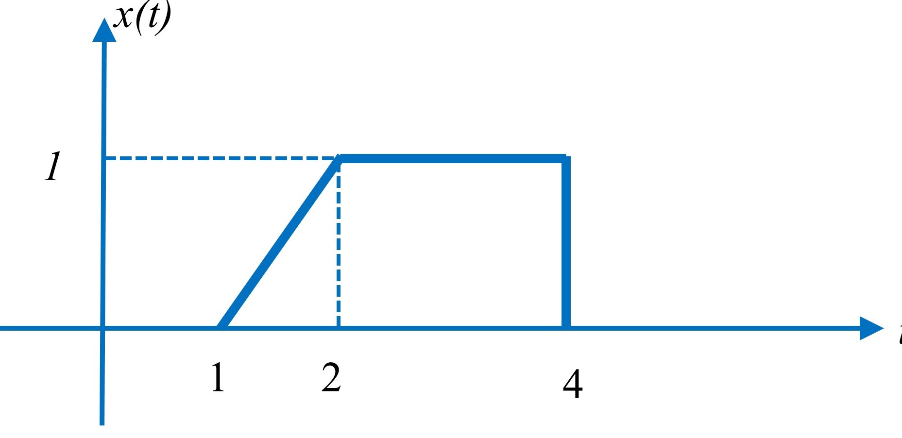
a) Write the signal description using the step and ramp functions. You will need to apply appropriate signal operations on the basic step and ramp functions to get x(t).
b) Now define x(t) in MATLAB and plot it.
c) Apply time-inverse operation to the signal (y(t)=x(-t)), and plot it.
d) Time-scale the signal y(t) by a factor of 0.2, name it z(t), and plot it.
e) Time-shift the signal z(t) by 4 seconds to the right, name it m(t), and plot it.
f) Plot n(t)=m(t)+x(t) .
6. Consider the following signals:
x(t)=t[u(t)-u(t-2)]+t[u(t+2)-u(t)]
y(t)=t[u(t)-u(t-2)]-t[u(t+2)-u(t)]
z(t)=t[u(t+1)-u(t-3)]
a) Define the signals x(t) and y(t) in MATLAB and plot them.
b) For each of these signals, determine if the signal is even, odd or neither.
