3 Modelling a shelter
Cubicles equipped with heaters such as the one shown in Figure 2.1 could be used as temporarily shelters to protect people in cold weather conditions.
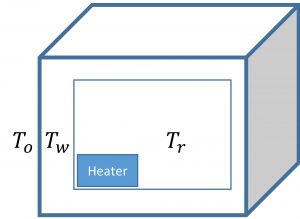
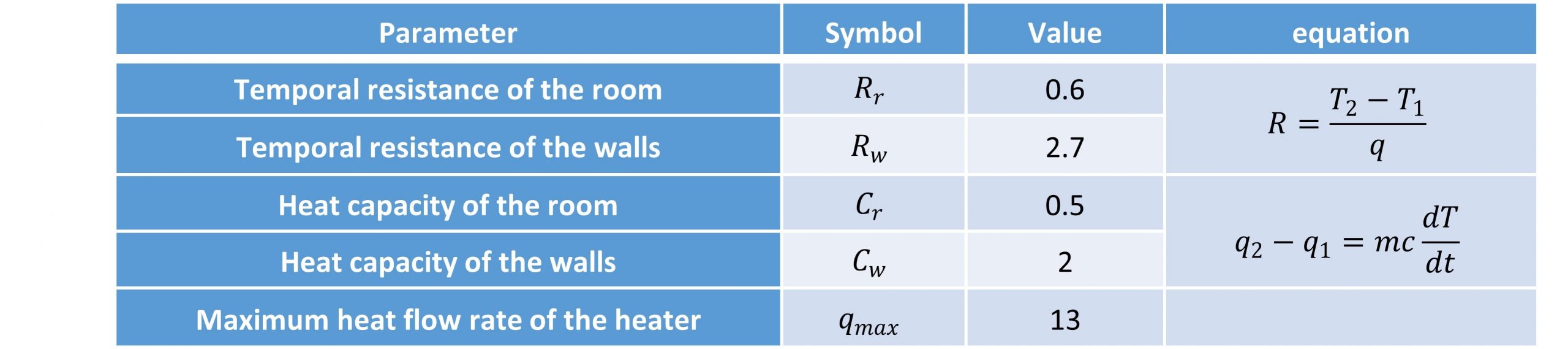
A company that builds such cubicles has provided a catalog as in Table 2.1. The purpose of this lab is to confirm the functionality of these cubicles in various conditions. Assuming the internal temperature of the cubicle is Tr, our goal is to adjust the heater to maintain this temperature in an appropriate range. The temperature of the walls is denoted as Tw , and the outside temperature is To ,which is considered as disturbance to the system because we do not have any control on the weather outside.
Table 1– Specifications of the cubicle
The heat flow rate of the heater is our input and control signal to the system. We will examine this system in different situations to see if it can provide our needs.
Objectives
The following objectives will be covered as you go through the experiment procedure.
- Examine the basic MATLAB functions
- Practice basic signals and operations
- Derive the the transfer function of a thermodynamic system
- Derive the state space of a thermodynamic system
- Derive the differential equations of a thermodynamic system
Procedure
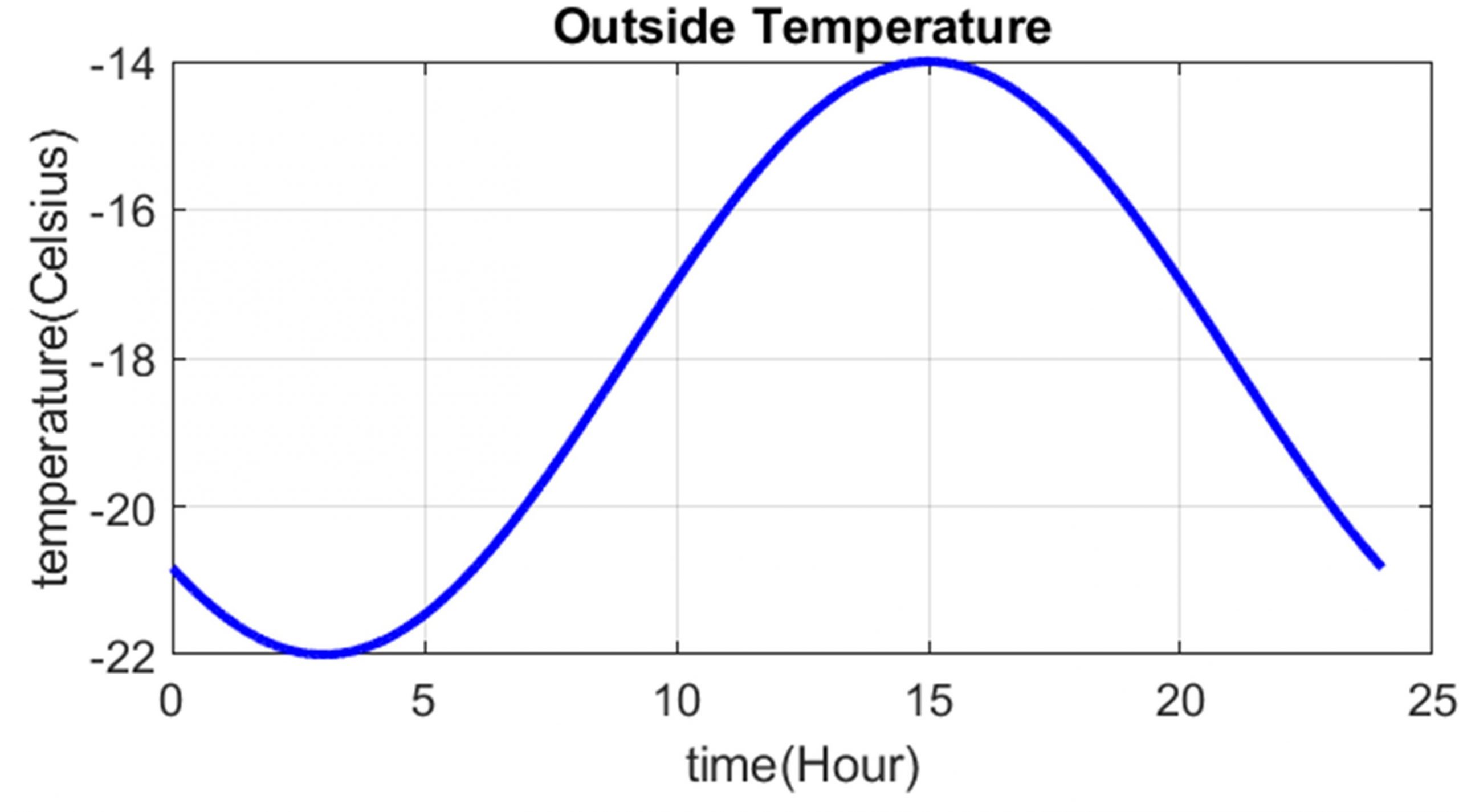
1. Assume Figure 2.2 shows the outside temperature To in a 24-hour cycle (one day). Write the function of the signal To (t) using signal operations (time shift, time scaling, and time-reversal) on the base signal F(t)=cos(t) . We assume that To waveform remains the same during our experiment.
2. Derive the differential equation that describes the relationship between the input (outside temperature Tr ) and output (internal temperature) of the system. Find the output ( Tr) for 3 days, by solving the differential equation with ode45 function in MATLAB (Solve Non-Stiff differential equations – medium order method) . Assume the heater turns on for the first time at midnight (Tr(0)=TW(0)=To(0)=0) and works with its maximum power instantly Q=qmax U(t).
3. Derive the transfer function of the system. Using the transfer function, simulate the system in MATLAB and derive Tr for the scenario described below. Then, plot Tr for 3 days. Note that is given in Part 1 and we don’t have any initial condition in the transfer function model. ( Tr(0)= D Tr(0)=0), where D represents x(t)=dx(t)/dt.
a) The heater turns on at midnight and reaches its nominal performance instantly (Q=qmax U(t) ). (Step signal) what if it happens in 10 hours? (Ramp signal)
b) The heater breaks and makes a big spark at 8 pm (Q=qmax Dirac(t-20) ) the next day. This situation will suddenly produce an amount of energy ( ) (Impulse signal).
c) Next, the heater doesn’t work for 10 hours. Imagine the heater slowly cools down (Q=qmax e-(t-20)) then it turns back on in the same way (Q=qmax (1- e-(t-30) ) )(Exponential signal).
4. Derive the state-space model of the system. Consider Tr, Tw as state variables, Tr as the output, Q as input, and To as a disturbance. Simulate the system in MATLAB. Try to derive the transfer function of the system from the state space. Verify that the transfer function obtained from the state space is the same as the one obtained in Part 3.
5. Assuming that the heater automatically turns off when the internal temperature reaches and turns on at (square signal), plot Tr for 3 days ( Tr(0) = Tw(0) = To(0) . Also, plot the internal temperature for 3 days if the temperature sensor has error (Noise).
