Topic 6: Consumer Theory
6.1 The Budget Line
Learning Objectives
- Understand budget lines
- Explain price ratios
- Recreate budget lines after prices and income changes
The Budget Line
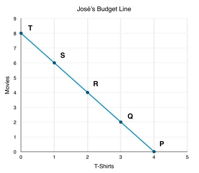
To understand how households make decisions, economists look at what consumers can afford. To do this, we must chart the consumer’s budget constraint. In a budget constraint, the quantity of one good is measured on the horizontal axis and the quantity of the other good is measured on the vertical axis. The budget constraint shows the various combinations of the two goods that the consumer can afford. Consider the situation of José, as shown in Figure 6.1a. José likes to collect T-shirts and movies.
In Figure 6.1a, the number of T-shirts José will buy is on the horizontal axis, while the number of movies he will buy José is on the vertical axis. If José had unlimited income or if goods were free, then he could consume without limit. But José, like all of us, faces a budget constraint. José has a total of $56 to spend. T-shirts cost $14 and movies cost $7.
Plotting the budget constraint is a fairly simple process. Each point on the budget line has to exhaust all $56 of José’s budget. The easiest way to find these points is to plot the intercepts and connect the dots. Each intercept represents a case where José spends all of his budget on either T-shirts or movies.
If José spends all his money on movies, which cost $7, José can buy $56/$7, or 8 of them. This means the y-intercept is the point (0,8). Here, José buys 0 T-shirts and 8 movies.
If José spends all his money on T-shirts, which cost $14, José can buy only 4 of them ($56/$14). This means the x-intercept is the point (4,0). Here, José buys 4 T-shirts and 0 movies.
By connecting these two extremes, you can find every combination that José can afford along his budget line. For example, at point R, José buys 2 T-shirts and 4 movies. This costs him:
T-Shirts @ $14 x 2 = $28
Movies @ $7 x 4 = $28
Total = $24 + $28 = $56
This point indeed exhausts José’s budget.
Budget Constraints
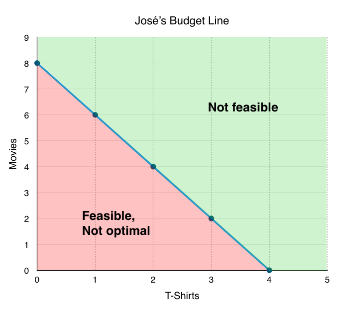
We now know that José must purchase at some point along the budget line, depending on his preferences. Note that any point within the budget line is feasible. José can spend less than $56, but this is not optimal as he can still buy more goods. Since T-shirts and movies are the only two goods, there is no ability in this model for José to save. This means that not spending his full budget is essentially wasted income. On the other hand, any point beyond the budget line is not feasible. If José only has $56, he cannot spend more than that. Notice that areas in the green zone are not necessarily more optimal than points along the budget line. The optimal point depends on José’s preferences, which we will explore when we discuss José’s indifference curve.
Slope
Though we can easily just connect the X and Y intercepts to find the budget line representing all possible combinations that expend José’s entire budget, it is important to discuss what the slope of this line represents. Remember, the slope is the rate of change. In economics, the slope of the graph is often quite important. In this situation, the slope is QY/QX. If we want to represent slope in terms of prices it is equal to Px/PY. This can seem unintuitive at first, as we are used to seeing slope as Y/X., but the reason this is not true for prices is because the y-axis represents quantity, not price. As we saw above, as price doubles, the quantity the consumer could previously purchase is halved.
If José is making $56:
When the price of movies is $7, he can buy 8 of them
When the price of movies is $14, he can buy 4 of them
Since price and quantity have this inverse relationship, we can use either Px/PY or QY/QX to find the slope. Since price is often the information given, it is important to remember that the slope can be calculated either way.
What Does Slope Mean?
The meaning of the budget line’s slope or price ratio is the same as the slope of a PPF. (The difference between these two curves is that the PPF shows all the different combinations given time a time/production constraint, whereas a budget line shows different combinations given budget constraint. Otherwise, the two graphs are basically the same). This means the slope of the curve is the relative price of the good on the x-axis in terms of the good on the y-axis. The price ratio of 2 means that José must give up 2 movies for every T-shirt. Likewise, the inverse slope of 1/2 means that José must give up 1/2 a T-shirt per movie.
When Income Changes
Because budget and prices are prone to change, José’s budget line can shift and pivot. For example, if José’s budget drops from $56 to $42, the budget line will shift inward, as he is unable to purchase the same number of goods as before.
To plot the new budget line, find the new intercepts:
Budget: $42
Price of movies: $7
Price of T-shirts: $14
Maximum number of movies (y-intercept): $42/$7 = 6
Maximum number of T-shirts (x-intercept): $42/$14 = 3
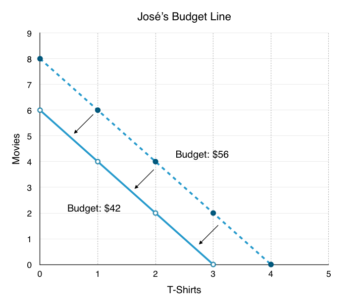
As a result of the shift, José’s budget line has shifted inward, leaving less consumption opportunities available.
When Price Changes
In addition to income changes, sometimes the prices of movies and T-shirts rises and falls. Suppose, from our original budget of $56, movies double in price from $7 to $14. Again, to plot the new graph, simply find the new intercepts:
Budget: $56
Price of movies: $14
Price of T-shirts: $14
Maximum number of movies (y-intercept): $56/$14 = 4
Maximum number of T-shirts (x-intercept): $56/$14 = 4
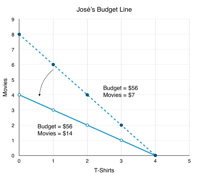
As a result of the pivot, José has fewer consumption opportunities available and the slope of the line changes. This has two effects:
The Size Effect: There are fewer opportunities for consumption (as a result of the price change, the purchasing power of José’s dollar has fallen).
The Slope Effect: The relative price of movies is now higher, while the relative price of T-shirts is now lower.
When Price and Income Change
The last type of change is when both price and income change. Suppose the price of movies increases from $7 to $12 and José’s budget increases to $63. To plot the new budget line, follow the same steps as before:
Budget: $63
Price of movies: $12
Price of T-shirts: $14
Maximum number of movies (y-intercept): $63/$12 = 5.25
Maximum number of T-shirts (x-intercept): $63/$14 = 4.50
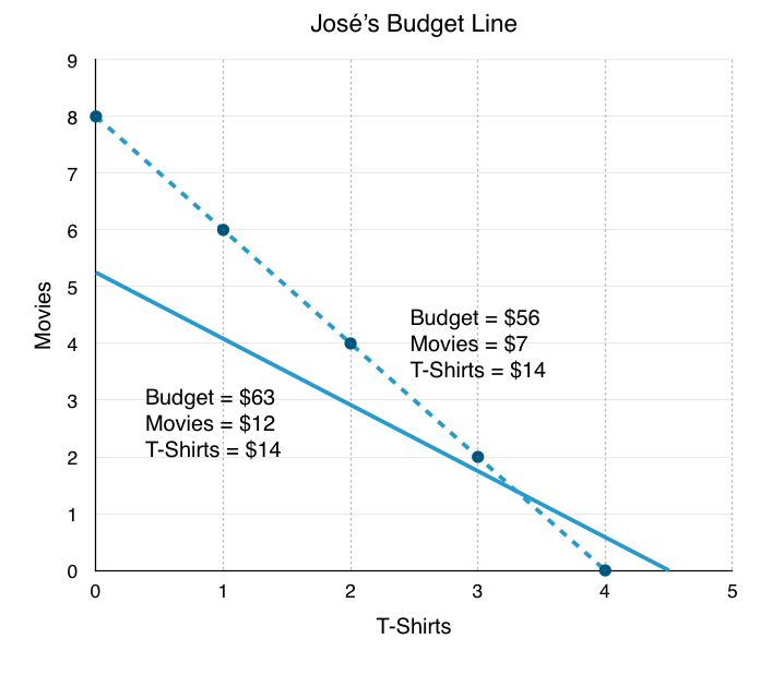
These changes have interesting effects. José now has access to some new consumption opportunities, but many others are now unavailable. While the slope effect has clearly made the relative price of T-shirts lower, the size effect is uncertain. These effects are implicit in the income and substitution effects we will explore shortly.
Conclusion
Though we understand the different ways by which consumers can exhaust their income, we have not yet discussed how to determine which bundles of goods different consumers prefer. To finish our analysis, let’s take a look at Indifference Curves.
Glossary
- Budget Constraint
- all possible combinations of goods and services that can be attained given current prices and limited income
- Budget Line
- a graphical representation of a consumers budget constraint
- Price Ratio
- the slope of the budget line, represents the price of x in terms of good y
- Size Effect
- the impact of a price change on the purchasing power of the consumer
- Slope Effect
- the impact of a price change on the relative prices of good x and y
Exercises 6.1
1. In the diagram below, a consumer maximizes utility by choosing point A, given BL1.
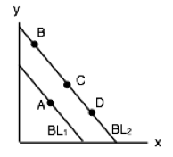
Suppose that both good x is normal and good y is inferior, and the budget line shifts to BL2. Which of the following could be the new optimal consumption choice?
a) B.
b) C.
c) D.
d) Either B or C or D.
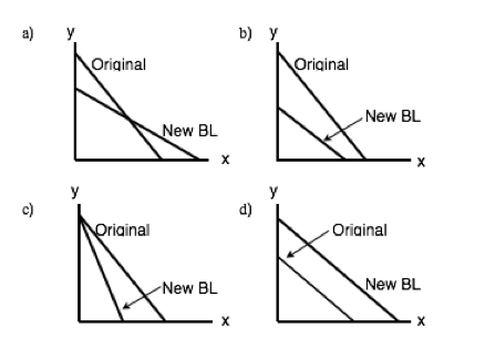
2. Which of the following diagrams could represent the change in a consumer’s budget line if (i) the price of good y increases AND (ii) the consumer’s income decreases.

Feedback/Errata