Topic 7: Producer Theory
7.1 Building Producer Theory
Learning Objectives
By the end of this section, you will be able to:
- Understand the relationship between marginal product of labour and marginal cost
- Derive average cost from marginal costs
- Represent a firm’s short run costs on a producer theory diagram
Different firms face different kinds of costs. A list of the costs involved in producing cars will look very different from the costs involved in producing fast-food meals. However, the cost structure of all firms can be broken down into some common types.
To start, we want to look at the costs of a single firm in the short run. These costs come from the different inputs required to produce a good, whether that is machines, labour, ingredients, rent, etc. By short run, we mean that there is at least one input that cannot be changed. This input (or inputs) is classified as a fixed cost since in the short term there is nothing we can do to avoid this cost except quit producing altogether.
When a firm looks at its total costs of production in the short run, a useful starting point is to divide total costs into two categories: fixed costs (ones that cannot change) and variable costs (ones that can change).
To guide our understanding of fixed and variable costs, consider Henry Ford once more. When Ford was opening his first factory, he had to consider different categories of costs.
Fixed Costs
Ford’s fixed costs are his expenditures that do not change regardless of his level of production. Whether he produced a lot or a little, his fixed costs are the same.
The first step for Ford to open his factory is finding the factory space. Ford must find someone who is willing to sell or rent him space. His first offer comes from Tom, who will only rent to Ford if Ford signs a 1-year lease for $20,000. Ford, with little negotiating power, agrees and signs the lease.
Once Ford signs the lease, the rent for the year costs him $20,000 regardless of how much he produces. This lease has now become a sunk cost since there is nothing Ford can do to get his money back. Fixed costs can take many other forms: for example, the cost of machinery or equipment to produce the product, research and development costs, even an expense like advertising to popularize a brand name. The level of fixed costs varies according to the specific line of business. For instance, manufacturing computer chips requires an expensive factory, but a local moving and hauling business can get by with almost no fixed costs at all if it rents trucks by the day when needed. Since Fords cost is fixed for a whole year, this is the length of his ‘short-run.’ During that period, since the lease expense is sunk, it should not affect his decision making.
Variable Costs
Ford’s variable costs are incurred in the act of producing—the more he produces, the greater the variable cost.
After signing the lease for the factory and purchasing machines, Ford now has to buy the raw materials and find workers to produce his cars. The more Ford wants to produce, the more workers and raw materials he will have to buy. For this reason, his variable costs are increasing as his production increases.
Marginal Product of Labour
For now, let’s diverge from the Ford example and consider an industry that is more labour intensive: barbershops. In the service industry, one of the most important variable costs is labour. How do we measure the cost of labour? It is not as simple as the hourly wage.
Consider a barbershop called “The Clip Joint.” For The Clip Joint, the variable costs include hiring barbers. Assume this cost is $80 per barber each day. The quantity of haircuts the barbershop can produce will increase as it hires additional barbers. Consider Table 1, which depicts the number of haircuts each new barber can produce. Notice that the first barber can only do 15 haircuts a day, whereas the next can cut 22.
| Number of Barbers | Number of Haircuts/New Barber |
| 1 | 15 |
| 2 | 22 |
| 3 | 25 |
| 4 | 23 |
| 5 | 19 |
| 6 | 13 |
This represents the Marginal Product of Labour, or the change in output that results from employing an extra unit of labour. The table can be depicted on a graph, with MPL on the y-axis and the # of Barbers on the x-axis. On the graph, we notice that at a certain level of barbers, our marginal gains from an extra barber begin to fall.
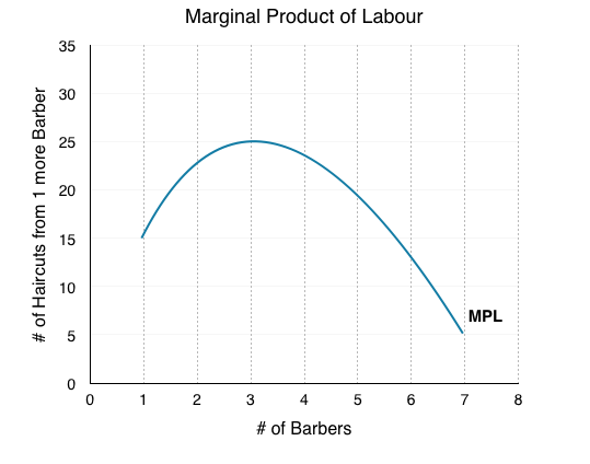
To understand the reason behind this pattern, consider that a one-man barber shop is a very busy operation. The single barber needs to do everything: say hello to people, answer the phone, cut hair, clean up, and run the cash register. A second barber reduces the level of disruption from jumping back and forth between these tasks, and allows a greater division of labor and specialization. The result can be greater increasing marginal returns. However, as other barbers are added, the advantage of each additional barber is less, since the specialization of labor can only go so far. The addition of a sixth or seventh or eighth barber just to greet people at the door will have less impact than the second one did. This is the pattern of diminishing marginal returns. As a result, the total costs of production will begin to rise more rapidly as output increases. At some point, you may even see negative returns as the additional barbers begin bumping elbows and getting in each other’s way. In this case, the addition of still more barbers would cause the output to decrease.
This pattern of diminishing marginal returns is common in production. As another example, consider the problem of irrigating a crop on a farmer’s field. The plot of land is the fixed factor of production, while the water that can be added to the land is the key variable cost. As the farmer adds water to the land, output increases. But adding more and more water brings smaller and smaller increases in output until at some point the water floods the field and reduces output. Diminishing marginal returns occur because we are ultimately constrained by some fixed factor.
Marginal Costs
How do we represent the MPL as a variable cost? Remember that the cost of hiring a barber is equal to $80/day. We want to find the cost per each additional unit of output. This is quite easy. If the first barber costs $80 to hire and can do 15 haircuts per day, then the marginal cost per haircut is equal to $5.33/haircut (Wage/MPL). This can be calculated for every level of output.
| Number of Barbers | Number of Haircuts/New Barber (MPL) | Cost/Haircut ($80/MPL) |
| 1 | 15 | $5.33 |
| 2 | 22 | $3.64 |
| 3 | 25 | $3.20 |
| 4 | 23 | $3.48 |
| 5 | 19 | $4.21 |
| 6 | 13 | $6.15 |
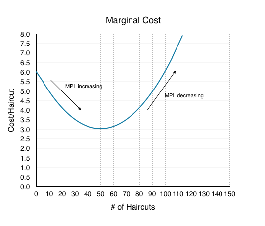
From this data, we can graph the marginal cost. Note that the x-axis has changed from 'Barbers' to 'Haircuts.' This is because whereas productivity is best understood in reference to the number of workers, marginal cost is defined for each level of output. You can see from Figure 7.1b that the marginal cost of the first haircut is $6.In our table, the cost per haircut of the first barber was only $5.33. Just as we can tell a story about the productivity increasing as we add more barbers, we can tell a similar story about the productivity increasing as a barber cuts more sets of hair. Our first barber may cut just one, or they may cut 15 heads. The $5.33/Haircut is the average of those first 15. The resulting cost curve is therefore a loose translation of the above table.
Notice that when marginal cost falls, it is because the inputs of production (in this case labour) are becoming more productive (MPL is increasing). When marginal cost is rising, it is because inputs are becoming less productive.
Average Variable Costs
We now have the first piece of producer theory. With information on marginal costs, we can use marginal analysis to determine whether increasing our inputs will be profitable. This is certainly important. In business, however, we often want to be able to answer “how much does a single haircut cost to produce”. Right now, our answer is “it depends” since our costs vary based on the number of barbers. Sometimes, we want to ignore this variation and calculate the average variable cost. Average variable cost is calculated by taking the total costs from every barber up to that point and dividing it by the total number of haircuts those barbers cut collectively.
Our average variable cost can be represented on the same graph as our marginal cost curve, helping us build our producer theory diagram even further.
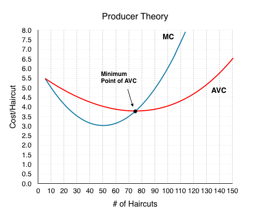
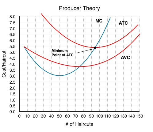
Notice that the marginal cost line intersects the average cost line exactly at the bottom of the average cost curve— this occurs at a cost of $4.0. The reason why the intersection occurs at this point is built into the economic meaning of marginal and average costs. If the marginal cost of production is below the average cost of producing previous units, as it is for the points to the left of where MC crosses AVC, then producing one additional unit will reduce average costs overall—and the AVC curve will be downward-sloping in this zone. Conversely, if the marginal cost of production for producing an additional unit is above the average cost of producing units, as it is for points to the right of where MC crosses AVC, then producing a marginal unit will increase average costs overall—and the AVC curve must be upward-sloping in this zone. The point of transition, between where MC is pulling AVC down and where it is pulling it up, must occur at the minimum point of the AVC curve.
When MC begins to increase, notice that AVC does not immediately increase. As long as marginal cost is below average cost, it causes AVC to decrease. When MC intercepts AVC and begins to rise, it causes AVC to increases. As we will see, AVCMIN is very important in the short run. See the application “Average Can Fall While Marginal Increases: Grades” to solidify this interaction.
Average Can Fall While Marginal Increases: Grades

This concept can seem confusing at first, but it in fact quite intuitive. Consider how you calculate your grades. If you are normally an A student and have an 80% average in Microeconomics, you will likely be disappointed if you received a 50% on a Midterm. Say, on the next midterm, you receive 65% – this is better than the 50% from last time but is still bringing you down from the A average you had hoped for. This is similar to the case of MC and AVC. MC is like the midterm grades – even when it is increasing, if it is still below your average, it will continue to bring it down, and when it is greater than average, it will bring it up.
Average Product of Labour
Backtracking slightly, the same analysis can be done for the Average Product of Labour, which can also be used to derive the AVC curve. Consider the graph below which represents the interaction between MPL and APL.
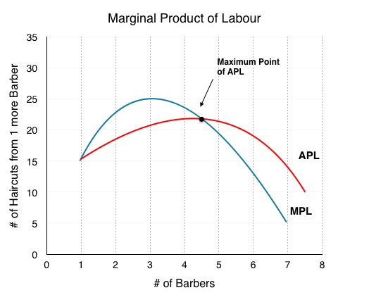
Notice that the maximum point on the APL happens at the same point (4.5 barbers) as the minimum point on AVC in Figure 7.1c. This is because when on average barbers are most productive, costs/haircut are lowest. Comparing the APL/MPL graph to the AVC/MC graph we see that the curves are inversely related.
Average Total Costs
We now have MC and AVC represented in our producer theory model. How do we represent fixed costs? Let’s assume the Clip Joint has fixed costs equal to $150 per day. average total cost is an average of our total variable cost and total fixed costs. As such, it can be found by (total VC + FC)/Q. Expanding this equation, we see it is equivalent to VC/Q+FC/Q which is AVC + AFC. Since we already have our AVC, all we have to do is add the FC/Q at each level of production.
Notice that we have changed the units on the x-axis of our producer theory graph from # of Barbers to # of Haircuts. Although in this example MC would be a constant $5.33 from 0 haircuts to 15 haircuts and constant $3.64 from 15 haircuts to 37 haircuts, in a larger market, this curve would be smoothed out. The following has been smoothed out to represent a different MC for each haircut.
So what is our ATC when we are producing 50 haircuts? Our AVC is $4.00. Our AFC at this point will be quite high at $150/50 = $3. This means our ATC is $4.00 + $3.00 = $7.00. Consider how AFC changes as we increase Q:
Q = 10 –> AFC = $150/10 = $15
Q = 20 –> AFC = $150/20 = $7.5
Q = 30 –> AFC = $150/30 = $5
Q = 150 –> AFC = $150/150 = $1
Since the only effect of an increase of inputs is spreading FC out amongst more units, AFC is always falling as Q increases.
Since AVC = ATC – (FC/Q), at low levels of Q, FC/Q is high. This means AVC is < ATC by a significant amount.
At high levels of Q, FC/Q is low. This means AVC is < ATC by a small amount.
As Q increases, FC/Q approaches 0 and AVC and AFC converge, as seen on Figure 7.1e
Why are total cost and average cost not on the same graph?
Total cost, fixed cost, and variable cost each reflect different aspects of the cost of production over the entire quantity of output being produced. These costs are measured in dollars. In contrast, marginal cost, average cost, and average variable cost are costs per unit. In the previous example, they are measured as cost per haircut. Thus, it would not make sense to put all of these numbers on the same graph, since they are measured in different units ($ versus $ per unit of output).
It would be as if the vertical axis measured two different things. In addition, as a practical matter, if they were on the same graph, the lines for marginal cost, average cost, and average variable cost would appear almost flat against the horizontal axis, compared to the values for total cost, fixed cost, and variable cost. Using the figures from the previous example, the total cost of producing 40 haircuts is $296, but the average cost is $296/40, or $7.4. If you graphed both total and average cost on the same axes, the average cost would hardly show.
A Variety of Cost Patterns
The pattern of costs varies among industries and even among firms in the same industry. Some businesses have high fixed costs, but low marginal costs. Consider, for example, an Internet company that provides medical advice to customers. Such a company might be paid by consumers directly, or perhaps hospitals or healthcare practices might subscribe on behalf of their patients. Setting up the website, collecting the information, writing the content, and buying or leasing the computer space to handle the web traffic are all fixed costs that must be undertaken before the site can work. However, when the website is up and running, it can provide a high quantity of service with relatively low variable costs, like the cost of monitoring the system and updating the information. In this case, the total cost curve might start at a high level, because of the high fixed costs, but then might appear close to flat, up to a large quantity of output, reflecting the low variable costs of operation.
For other firms, fixed costs may be relatively low. For example, consider small businesses that rake leaves in the fall or shovel snow off sidewalks and driveways in the winter. For fixed costs, such firms may need little more than a car to transport workers to customer’s homes and some rakes and shovels. Still other firms may find that diminishing marginal returns set in quite sharply. If a manufacturing plant tried to run 24 hours per day, seven days a week, little time remains for routine maintenance of the equipment, and marginal costs can increase dramatically as the firm struggles to repair and replace overworked equipment.
Every firm can gain insight into its task of earning profits by dividing its total costs into fixed and variable costs, and then using these calculations as a basis for average total cost, average variable cost, and marginal cost. However, making a final decision about the profit-maximizing quantity to produce and the price to charge will require combining these perspectives on cost with an analysis of sales and revenue, which in turn requires looking at the market structure in which the firm finds itself. Before we turn to the analysis of market structure in other topics, we will analyze how a perfectly competitive firm makes decisions in the short- and long-run
Key Concepts and Summary
In the short-run, a firm’s total costs can be divided into fixed costs, which a firm must incur before producing any output, and variable costs, which the firm incurs in the act of producing. Fixed costs are sunk costs; that is, because they are in the past and cannot be altered, they should play no role in economic decisions about future production or pricing until out short run’s time horizon is up. Variable costs typically show diminishing marginal returns, so that the marginal cost of producing higher levels of output rises.
Marginal cost is calculated by taking the change in total cost (or the change in variable cost, which will be the same thing) and dividing it by the change in output for each level. Marginal costs are typically rising. A firm can compare marginal cost to the additional revenue it gains from selling another unit to find out whether its marginal unit is adding to its profit.
Average total cost is calculated by taking total cost and dividing by total output at each different level of output. Average costs are typically U-shaped on a graph.
Average variable cost is calculated by taking variable cost and dividing it by the total output at each level of output. Average variable costs are also typically U-shaped.
Glossary
- Average Product of Labour
- the average amount of output each worker can produce; Total product/Total output
- Average Total Cost
- total cost divided by the quantity of output
- Average Variable Costs
- ariable cost divided by the quantity of output
- Diminishing Marginal Returns
- the decrease in the marginal output of a production as input is is incrementally increased
- Fixed Cost
- expenditure that must be made before production starts and that does not change regardless of the level of production
- Marginal Product of Labour
- the amount of output an additional worker can produce
- Short Run
- a period of time in which at least one cost factor is fixed
- Total Cost
- the sum of fixed and variable costs of production
- Variable Costs
- cost of production that increases with the quantity produced
Exercises 7.1
The following FOUR questions refer to the table below, which shows the relationship between labour and output for a firm.
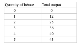
1. The marginal product of the fourth unit of labour hired is:
a) 10.
b) 3.
c) 4.
d) 0.
2. If each unit of labour must be paid a wage of $10, then what do (total) variable costs equal, at an output level of 25 units?
a) $250.
b) $50.
c) $20.
d) $2.
3. If three workers are employed, then the average product of labour is:
a) 12.
b) 11.
c) 36.
d) 40.
4. If each unit of labour must be paid a wage of $12, then what is the marginal cost of the 43rd unit of output?
a) $12.
b) $36.
c) $3.
d) $4.
5. Suppose that the marginal produce of labour is always decreasing in number of workers employed. Which of the following statements about the marginal cost of producing output is true?
Which of the following statements is true?
a) Marginal cost is constant in output.
b) Marginal cost is decreasing in output.
c) Marginal cost is increasing in output.
d) Marginal cost is decreasing in output at low level of output, and increasing in output at high levels of output.
6. If the marginal cost of producing output is constant and equal to $5 per unit, and fixed costs are equal to $600, then average total cost given an output level of 100 is:
a) $5.
b) $6.
c) $11.
d) $20.

Feedback/Errata