Topic 3: Supply, Demand, and Equilibrium
Solutions: Case Study – The Housing Market
1. Label Figure CS3 a. with the Equilibrium price and quantity, and label supply and demand curves as either renters or landlords.
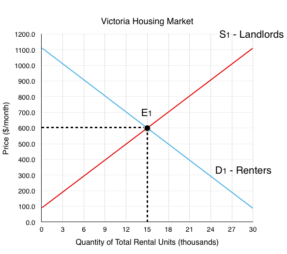
Since Landlords supply the housing units, they represent the supply side of the market, labeled S1.
Since Renters demand the housing units, they represent the demand side of the market, labeled S2.
The equilibrium E1 occurs at the intersection of supply and demand, in this case @ EP1 = $600, EQ1 = 15,000 rental units.
2. Explain why a housing market at equilibrium could still have a vacancy rate of 4%.
In a perfect equilibrium, the housing market would have no vacancies. However, one of the requirements of a perfect equilibrium is a instant transmission of information. In the real market, this is not the case. Because of this, even if there is an equal amount of supply and demand, it is difficult for renters to match up with landlords. This means that when someone leaves the rental market, it takes time before that vacancy is filled. Therefore even when supply = demand there can be a positive vacancy rate in the market. Depending on the speed of information transfer, there will be an equilibrium vacancy rate that represents healthy market conditions – without further information we could assume this rate is around the Canadian average of 3.3%. This means that a vacancy rate of 0.6% would have to represent a shortage of housing from disequilibrium.
3. Assume 3000 landlords decide to switch from renting to Airbnb, show the impact of the changes on Figure CS3 b. Label the new equilibrium price and quantity.
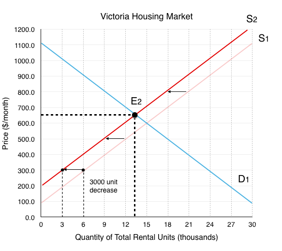
The decrease in landlords causes a decrease in supply. We can find the exact magnitude of the shift by looking at how much quantity supplied decreases for each price level. In this case, we are told to assume that quantity supplied decreases by 3000 rental units at every price. This causes a shift from S1 to S2.
The new equilibrium E2 results from the intersection between S2 and D1, in this case @ EP2 = $650, EQ2 = 13,000 rental units.
4. Assume 9000 new renters enter the market instead of mortgaging homes, show the impact of the changes on Figure CS3 b. Explain the impact of both the shock from Airbnb and the shock from less housing buyers on equilibrium price and quantity. Do the shocks work together or oppose one another?
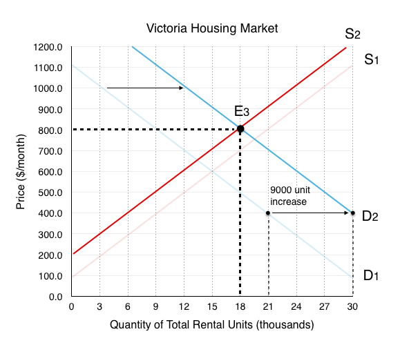
The increase in renters in the market causes an increase in demand. Again, the magnitude of the shift is given to us. We are told that quantity demanded increases by 9000 rental units at every price. this causes demand to shift from D1 to D2.
The new equilibrium E3 results from the intersection between S2 and D2, in this case @ EP3 = $800, EQ3 = 18,000 rental units.
We can see that compared to EP1 = $600, EQ1 = 15,000 rental units, E3 has seen a increase in price and quantity. Breaking down the two effects:
The decrease in supply caused price to rise and quantity to fall.
The increase in demand caused price to rise and quantity to rise.
We can see that the effects on price worked together, but the effects on quantity opposed. The end result of an increase in quantity is because the demand shock was greater than the supply shock. In this topic we explained that unless you know which effect is greater, the result of opposing shocks are inconclusive. In this case we can say with certainty that quantity has increased because we know the exact size of the shocks.
5. Assume price remains at the original equilibrium , calculate the magnitude of the shortage or surplus of housing that results. Explain the impact this shortage will have the behaviour of landlords.
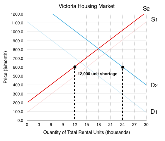
If price remains at the original equilibrium E1 of $600, Quantity Demanded @ D2 is 24,000 and Quantity Supplied @ S2 is 12,000. This means that there will be a 12,000 unit shortage in rental housing (24,000 – 12,000). As mentioned in the case study, this will cause pressure for prices to increase. Since landlords cannot raise prices for existing tenants, they will be incentivized to find ways to evict tenants. For the spots that are up for rent, bidding wars will ensue.
6. Assume the government wants to bring price back to it’s original level, if it costs $50,000 to increase the number of rental units by one, how much will this cost the government?
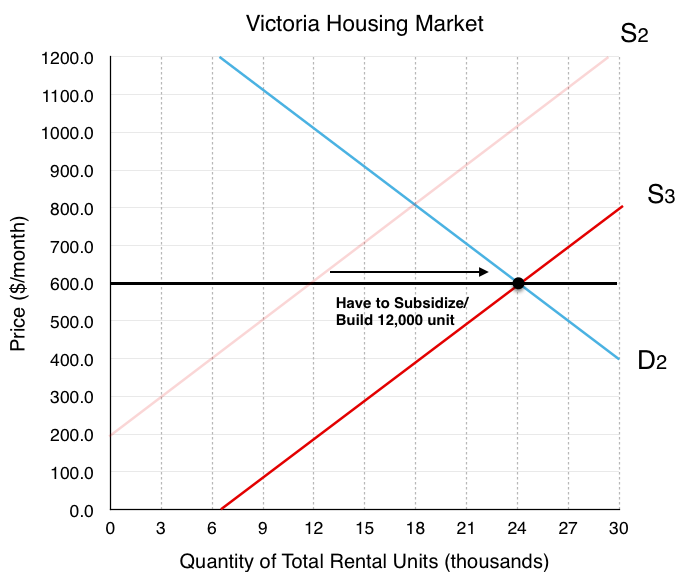
In order to shift supply from S2 to a supply curve that intersects with D2 at an equilibrium price of $600, the government has to find a way to increase the supply of rental housing by 12,000 units. If it costs $50,000/unit, this would cost the government $600 million.
7. Read the Executive Summary of the Alliance of BC Students White Paper on Student Housing. What is the ABCS proposing that could help decrease price in the market? How would this affect supply and/or demand?
The ABCS white paper draws attention to the fact that universities are currently restricted from accruing debt to build more student housing. They recommend that the government remove this restriction, explaining that the increase in housing for students will take them out of the competitive market above. Depending on how you view the market this could be explained as an increase in supply or a decrease of demand. If you consider student housing as a separate market, this effect would decrease demand as it takes student out of the market. If you consider it as the same market, it would increase supply as it increases the amount of housing available.

Feedback/Errata