Chapter 7. Geological Structures Part A: Relative Age and Orientation of Geologic Layers
Overview of Relative Age and Orientation of Geologic Layers
Block Diagrams
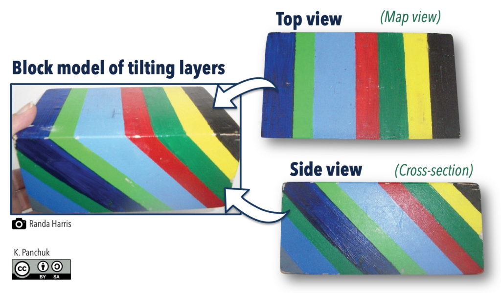
Geological structures exist in three dimensions, so it’s helpful to have a way of showing 3-D structures. Block diagrams are images that represent 3-D models of geological structures, and may be actual blocks of wood (Figure 7.1, left) or boxes of paper with geological structures marked on them.
Block models provide different information depending on how you view them. Viewed from above, the models represent what you’d see on a geological map. Viewed from the side, you see the cross section of the model. The side view is akin to the view you would get of geological structures if you drove through the mountains where roads have been cut through the rocks.
Cross-Section Views Let Us Interpret the History of Rocks
Often, part of the task of studying geological maps and drawings is to figure out how rocks have changed over time. Under the influence of gravity, sediments are deposited in horizontal layers, meaning that sedimentary rocks all start out as horizontal beds, as illustrated in the side view of the block model in Figure 7.2. This is called the principle of original horizontality. In a stack of sedimentary rocks, the oldest rocks will be on the bottom (because they had to be there first for the others to deposit on top of them), and the layers get younger moving up. This is called the principle of superposition. We can indicate the relative ages of the rocks (i.e., which are older and which are younger) by numbering them in the order in which they formed, with 1 being the oldest.
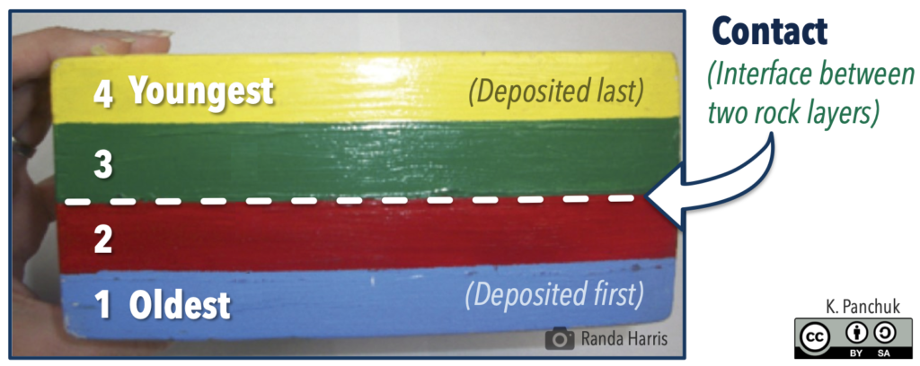
Boundaries between rock units are called geological contacts (in other words, contacts are where rocks are in contact with each other). In Figure 7.2, the contact between layers 2 and 3 is marked with a dashed line, but the boundary between layers 1 and 2, and between 3 and 4 are also contacts.
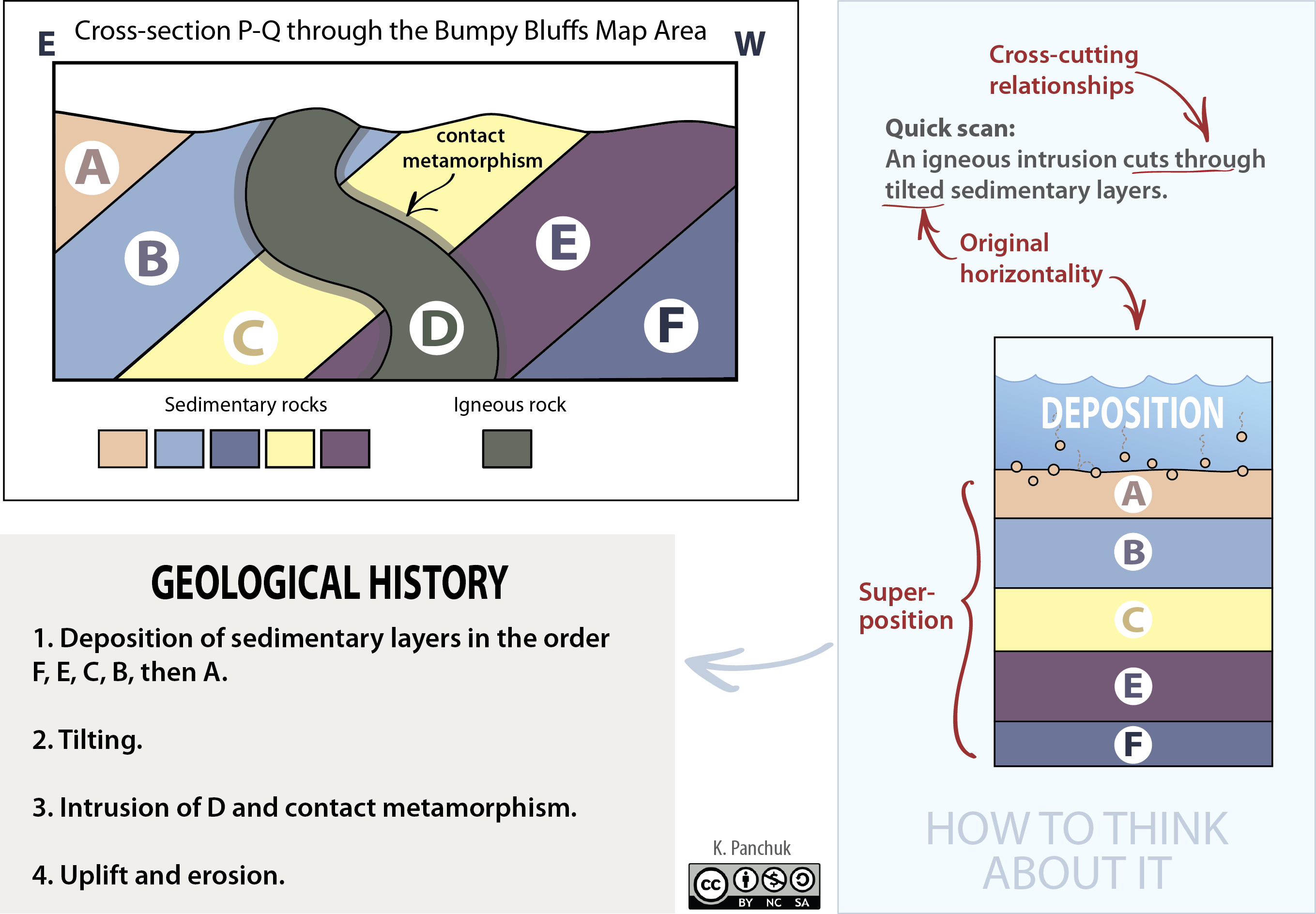
Figure 7.2 represents the most basic arrangement of sedimentary rock layers—a horizontal stack—but Earth’s layers are often more complicated than that. Layers may be tilted at an angle, as represented by the model in Figure 7.1. The law of original horizontality tells us that tilted sedimentary layers must have been re-oriented from their original horizontal position, such as by plate tectonic forces. We can still apply the law of superposition to determine which of the layers is oldest, by imagining how the layers would have been arranged before they were tilted. Assuming the layers have not been completely overturned (we assume they haven’t been, unless we have specific information saying otherwise), the grey bed in the lower left is the oldest.
Of course, the principle of horizontality does not apply to igneous intrusions, because their shape is determined by interaction with surrounding rock, and superposition does not necessarily apply, because igneous intrusions can be injected at various levels within Earth’s crust. With igneous intrusions and structures like faults (created by breaking and shifting of rocks), we can apply the reasoning that if a rock or structure cuts through another rock or structure, it must have formed after the rock that’s being cut. (You can’t slice a cake unless the cake is there first). This idea is called the principle of cross-cutting relationships.
How to Give the Geological History of Rocks Represented by a Cross-section
For purposes of this lab, “geological history” refers to the simplest sequence of events that could produce the arrangement of rocks shown on a geological map or in a cross-section. This can usually be accomplished by selecting one or more events from the list below, and arranging them in the correct order by applying the principles described above (original horizontality, superposition, cross-cutting relationships). For these lists of events, it isn’t necessary to add explanations of why or how the events occurred. The goal is a brief point-form list, like the one in Figure 7.3.
1. Deposition. Sedimentary layers and lava flows are deposited. If there is a stack of sedimentary layers, list the order in which they were deposited from oldest to youngest.
2. Intrusion and contact metamorphism. This applies to intrusive igneous rocks. A zone of contact metamorphism will be present anywhere igneous rocks (intrusive or extrusive) have touched pre-existing rocks.
3. Tilting. When sedimentary layers are dipping. Titling applies to all of the rocks that have been deposited up to that point, so you don’t need to say which ones were involved.
4. Folding, if rocks are folded rather than simply tilting. Note that tilted rocks might actually be folded, but on a larger scale than the cross-section. However, you should reserve “folding” for when folding is visible in the cross-section.
5. Faulting. Faults will be visible as offsets in rock layers.
6. Uplift and erosion. Tectonic uplift raises rocks above where deposition occurs. Erosion might be visible at the top of the diagram as hills and valleys carved into the rock layers, or as cut-off rock layers within the cross-section.
Folding and faulting will be discussed in more detail in the next chapter.
The following (Figure 7.3) is an example of the reasoning process for coming up with the geologic history, and how you would describe it.
Strike and Dip: Describing the Orientation of Rock Layers
Strike and dip are two parameters used to measure the orientation of rock layers. To get an intuitive sense of what they mean, have a look at the roof of the structure in Figure 7.4. If we needed to describe the orientation of the side of the roof above the long wall with three windows, we might start by identifying how the wall with windows or the ridge of the roof are oriented. According to the direction arrows in the photo, the ridge runs north-south. Next we would need to say how steep the roof is, and we could describe that in terms of how far off the roof is from being horizontal.
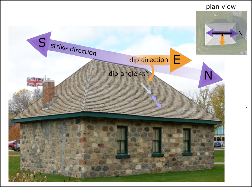
For geological layers, the strike is analogous to the direction the roof ridge is running. It is defined as the intersection of a horizontal plane and an inclined surface. You can visualize this as the line formed where the tilted rock layer in Figure 7.5 meets the surface of the lake. Dip is the angle between that horizontal plane (such as the water surface in Figure 7.5) and the inclined surface (such as a geological contact between tilted layers), measured perpendicular to the strike line down towards the inclined surface.
When describing the orientation of the side of the roof, one more piece of information is needed, because if we said the roof was running north-south and was tilted 45º down from horizontal, that would apply to the side of the roof on the opposite side of the house, as well as to the side we can see directly. We use the dip direction to indicate the downhill direction in map view. In the roof example, rain landing on the side of the roof facing us would run down the roof toward the east.
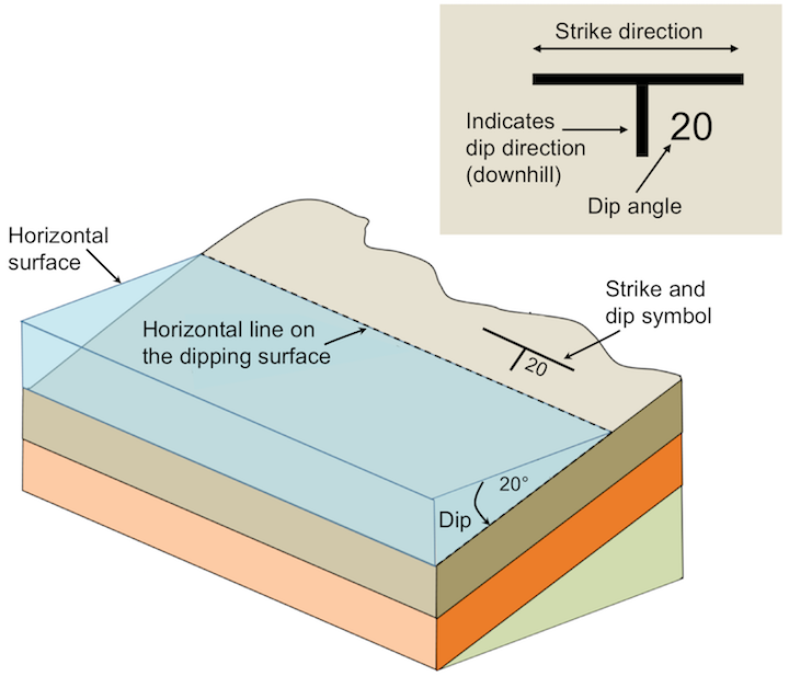
On a geological map, information about the bed orientation is provided using a T-shaped symbol, as shown on the surface of the bed in Figure 7.5. The top of the T is stretched out along the strike direction, and the vertical part points in the dip direction. The dip angle is written next to the symbol.
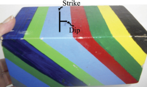
Now, let’s apply this concept to the block model of dipping beds (Figure 7.6). To find a strike line, find where a contact intersects the horizontal surface. The top of the block model is horizontal, and most of the beds on the model reach the top of the block, so there are many places to look for strike lines. The long part of the strike and dip symbol has been drawn parallel to the contacts. (It is usually drawn on a rock layer, not on a contact.) To determine dip direction, pretend that you are able to pull the model apart where the red and blue beds are touching, and put a drop of water on the blue bed. Which direction would the water flow if it followed that contact? That is the direction of dip. In this case, the dip direction is toward the right side of the figure. Note that the dip part of the symbol (shorter line) is always drawn perpendicular to the strike symbol, whatever the angle of dip.
Strike of a Horizontal Layer
The strike of a bed is defined by its intersection with a horizontal plane, but what if the bed is a horizontal plane? In the scenario where the dip is 0º, you could draw an infinite number of lines in an infinite number of orientations, so the concept of a strike simply isn’t meaningful for horizontal layers. We say that horizontal layers don’t have a strike, or that the strike is undefined.
Reporting Strike and Dip
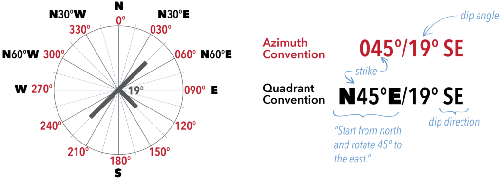
The notation for reporting strike and dip can take two forms. In both cases the dip is reported as a dip angle and dip direction, but the notation for strike differs. In the azimuth convention, compass directions are broken down into 360 degrees, and geographic directions are specified using three-digit numbers (Figure 7.7, red text). Due east is represented as 090º, for example as it represents a 90-degree angle from due north in a clockwise rotation. In the quadrant convention, geographic directions are described relative to how far away they are from the cardinal directions. The strike and dip symbol in Figure 7.7 has a strike of 045° in the azimuth convention, and N45ºE (understood as 45° East of due North) in the quadrant convention. Note that strikes go in both directions, meaning that a strike of 045º is the same as a strike of 225º or S45ºW. (The choice of strike direction is handled differently if you are using a right-hand rule, which we do not, and with good reason. Click here to jump to an explanatory footnote.)
Measuring Strike from a Map
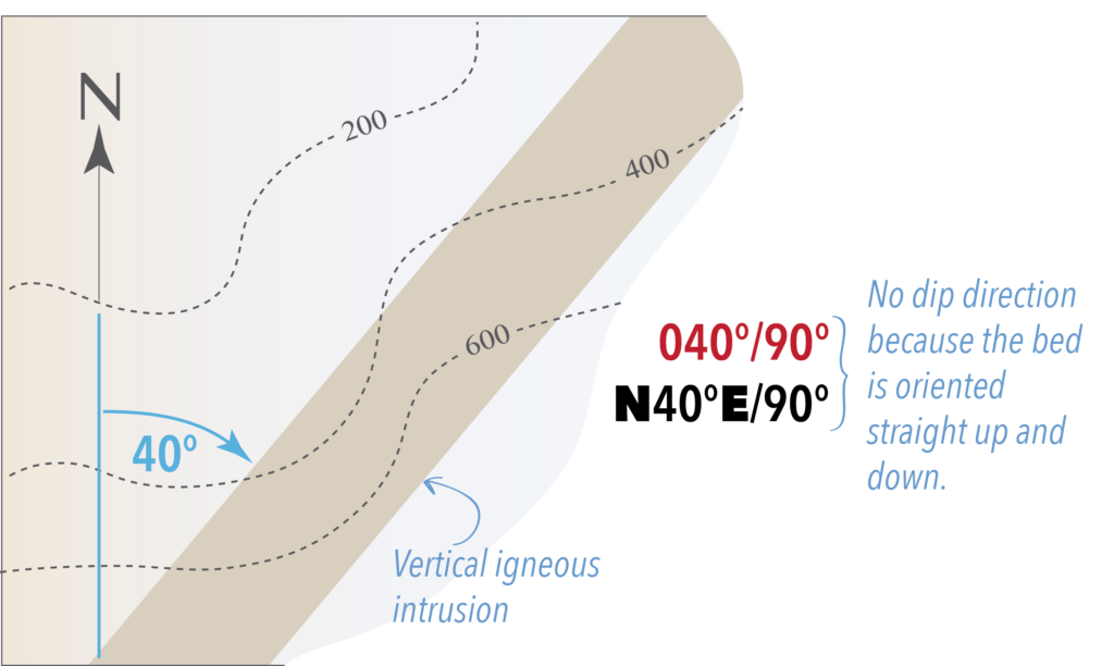
In many cases strike cannot be measured directly from the map without applying some geometric methods since the beds run at an angle. Vertical beds are an exception to this, however. You can measure the strike of a vertical bed by measuring the angle between one of the bed’s contacts and the north arrow (or a convenient feature with a known orientation). In Figure 7.8, a line has been extended down from the north arrow to the contact of the bed. The angle between the north arrow and the bed is 40°. The strike of the bed is therefore 040° (also N40ºE, 220°, S40°W).
Do you understand strike and dip well enough to solve this mystery and summon a cursed village back from the Nonverse?
Rock Layer Orientation and the Rule of Vs
You’ve used the rule of Vs when interpreting topographic maps, but there is a more advanced version that is useful for interpreting the direction in which beds or geological structures such as faults are tilted on maps. You can usually determine the dip direction of inclined beds by looking at whether a V forms, and in what direction it points, when the beds cross a valley on a map.
If an inclined bed dips in the opposite direction as the slope of the valley (Figure 7.9 A), the V will point in the direction of dip. The situation is more complex when the beds dip in the same direction that the valley slopes. If the dip of the beds is steeper than the slope of the valley (Figure 7.9 E), then the V will point in the direction of dip. But if the valley slopes steeper than the dip of the beds, the V will point in the opposite direction of dip (Figure 7.9 C). In the case where the stream/valley gradient is the same as the dip of the bed(Figure 7.9 D), the beds will run parallel on both sides of the valley.
For vertical beds, no V shape is created in map view: the bed cuts directly across the valley without being deflected in either direction (Figure 7.9 F). For horizontal beds, the edge of the bed will intersect topography parallel to topographic contours. If the landscape is sloping near the valley, the bed will generate a V shape parallel to the contour lines in the valley (Figure 7.9 B). If the landscape is flat near the valley, the bed will show up on both sides of the valley (Figure 7.10 I), similar to the case where the gradient of the bed equals the slope of the valley (Figure 7.9 D).
Vertical and Horizontal Beds
In the rule of Vs, vertical and horizontal beds generate unique patterns when they intersect with the surface of Earth. Figure 7.10 provides another illustration of characteristic patterns, this time for a symmetrical hill. In the case of the vertical beds (Figure 7.9F, 7.10G), there are no Vs produced in the landscape, and the feature is linear across the landscape despite the changes in the topography. (We would see the same pattern in the landscape for vertical faults or other vertical geological features.) In the case of horizontal beds (Figure 7.9 B, I; 7.10H), the strata intersect with the topography in lines that are parallel to the contour lines.
Geological Maps & Cross-Sections
A geological map uses lines, symbols, and colors to communicate information about the nature and distribution of rock units within an area. The map includes information about geological contacts and their strikes and dips. Geologists make these maps by careful field observations at numerous outcrops (exposed rocks at Earth’s surface) throughout the mapping area. At each outcrop, geologists record information such as rock type and the strike and dip of the rock layers. They can also include relative age data in their map if they are able to find evidence of relationships between the rocks using the principles of relative dating. Geological maps take practice to understand, because three-dimensional features (including complex features such as folds) are displayed on a two-dimensional surface. Remember that a geological map will be seen in map view (i.e., viewed from above). A geological map is analogous to viewing the floor plan of a house: there are many things you can represent in plan view (e.g., doors, appliances, stairs) that will help you visualize what the interior will look like if you were to visit the house in real life.
Geologists use information about rocks that are exposed to visualize how the unseen rocks beneath the surface are oriented. This allows geologists to prepare their best interpretation of the cross-sectional view of the geology below the surface, similar to what we observed in the blocks above.
A geological cross-section shows geologic features from the side view. The side views of the block models in Figures 7.1, 7.2, and 7.6 are cross-sections. Cross-sections are built on the topographic profiles that you created for topographic maps by adding rock types and geologic structures present beneath Earth’s surface.
LOTS: Legend, Orientation, Title, Scale
Every geological cross-section must include a legend, the orientation of the line the cross-section represents on the map, a title, and a scale (Figure 7.11). To help us remember, we abbreviate these four key parts with the acronym LOTS.
Legend: The legend is a key to the patterns used to identify each unit on the cross-section. The units are ordered from oldest formation at the bottom of the legend to youngest unit at the top of the legend.
Orientation: The orientation of the cross-section is the direction that the cross-section line makes on Earth (the “strike” direction of the cross-section line on the geological map). You can indicate the orientation by writing the corresponding direction at each end of the cross-section (e.g., west and east in Figure 7.9C).
Title: A descriptive title for the cross-section. You can include the letters used to identify the line on the original geological map in the title (e.g., “Cross-Section along Line X-Y”).
Scale: Include a ratio scale and/or a bar scale to show the scale of the cross-section. The vertical and horizontal scales should be the same, so you only need to include one scale on the cross-section.
How to Draw a Cross-Section
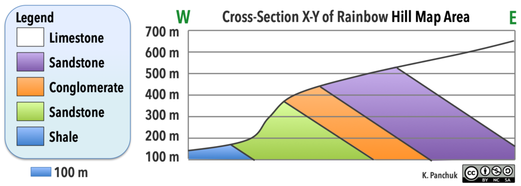
Advance through the slides to see the step-by-step process for constructing the cross-section in Figure 7.11 from the Rainbow Hill geological map. You can see a summary of the steps below.
Summary of steps for constructing a cross-section:
1. Examine the geological map that you are using to construct your cross-section, paying close attention to any strike and dip symbols, geological contacts, and ages of the rock types.
2. Find the position on the map designated for the cross-section. The line (called a transect) will be indicated by an actual line, or with positions labelled with letters on the edges of the map, such as “X” and “Y”.
3. Take a clean sheet of paper, and construct a topographic profile: Draw a box with horizontal lines for elevations, mark off each elevation that the transect goes through, then join the points with a smooth line. When drawing topographic profiles for constructing a cross-section, do not use vertical exaggeration.
4. Transfer the locations of the contacts to the topographic profile. Draw the contacts by extending lines below the profile at the correct angle measured down from the horizontal. Note: If beds are vertical or horizontal, there might not be a strike and dip symbol on the map. Use the patterns discussed in Figure 7.9 to help you decide if the beds are horizontal or vertical.
5. Don’t forget LOTS! Add a legend, orientation, title, and scale to your cross-section If possible, use the same colour scheme or pattern as the geological map.
Calculating Bed Thicknesses
You might have noticed in the explanations for drawing the cross-section in Figure 7.11 that the width of the beds on the geologic map aren’t the same as the thickness of the beds when viewed in cross-section. This is a common feature of many geological maps—generally, beds look wider in map view, and thinner in the cross-section. This happens when tilted beds are sliced and exposed by erosion at Earth’s surface. The width of a bed visible in map view that doesn’t represent the bed’s actual thickness is called the apparent thickness. (Figure 7.12. top). The bed’s actual thickness—its true thickness— is the thickness measured by drawing a line which intersects the top surface (upper contact) and bottom surface (lower contact; Figure 7.12, bottom) at a right angle.
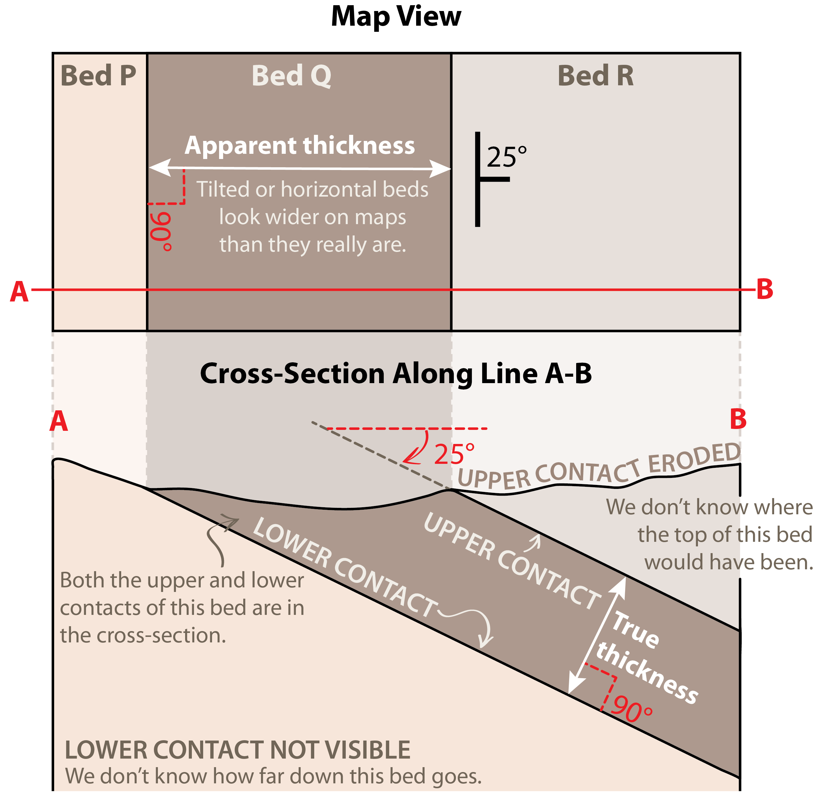
Note that while we can measure the true thickness of Bed Q, because both upper and lower contacts are present, we can’t measure the true thickness of Bed P or Bed R. Only one contact is visible for each. We can estimate a minimum thickness for Bed R by measuring at a right angle to the contact until it hits the eroded surface. We can’t do this for Bed P, however. If we measure to where the cross-section ends, what we get is just a function of how deep we’ve drawn our cross-section. For all we know, there could be another bed starting just a little to the left of the map edge that would show up in our cross-section if it were wider. From the limited information we have, we can’t rule out the possibility that Bed P is actually thinner than Bed Q.
Steps for Measuring True Thickness from a Cross-Section
You can measure the true thickness directly from a cross-section, provided that you drew your cross-section without vertical exaggeration (i.e., the vertical scale is the same as the map scale), and that the cross-section is drawn perpendicular to the strike of the beds (or, parallel to the dip direction):
- Measure the distance between the bottom of the bed (lower contact )and the top of the bed (upper contact). Be sure to measure at right angles to the contacts. (See the arrow labelled “true thickness” in Figure 7.12).
- Apply the scale of the cross-section to get the true thickness. For example, if the cross-section is drawn to a scale of 1 cm = 100 m and you measure a distance of 2.4 cm between contacts, the thickness is 2.4 cm x 100 m/1 cm = 240 m.
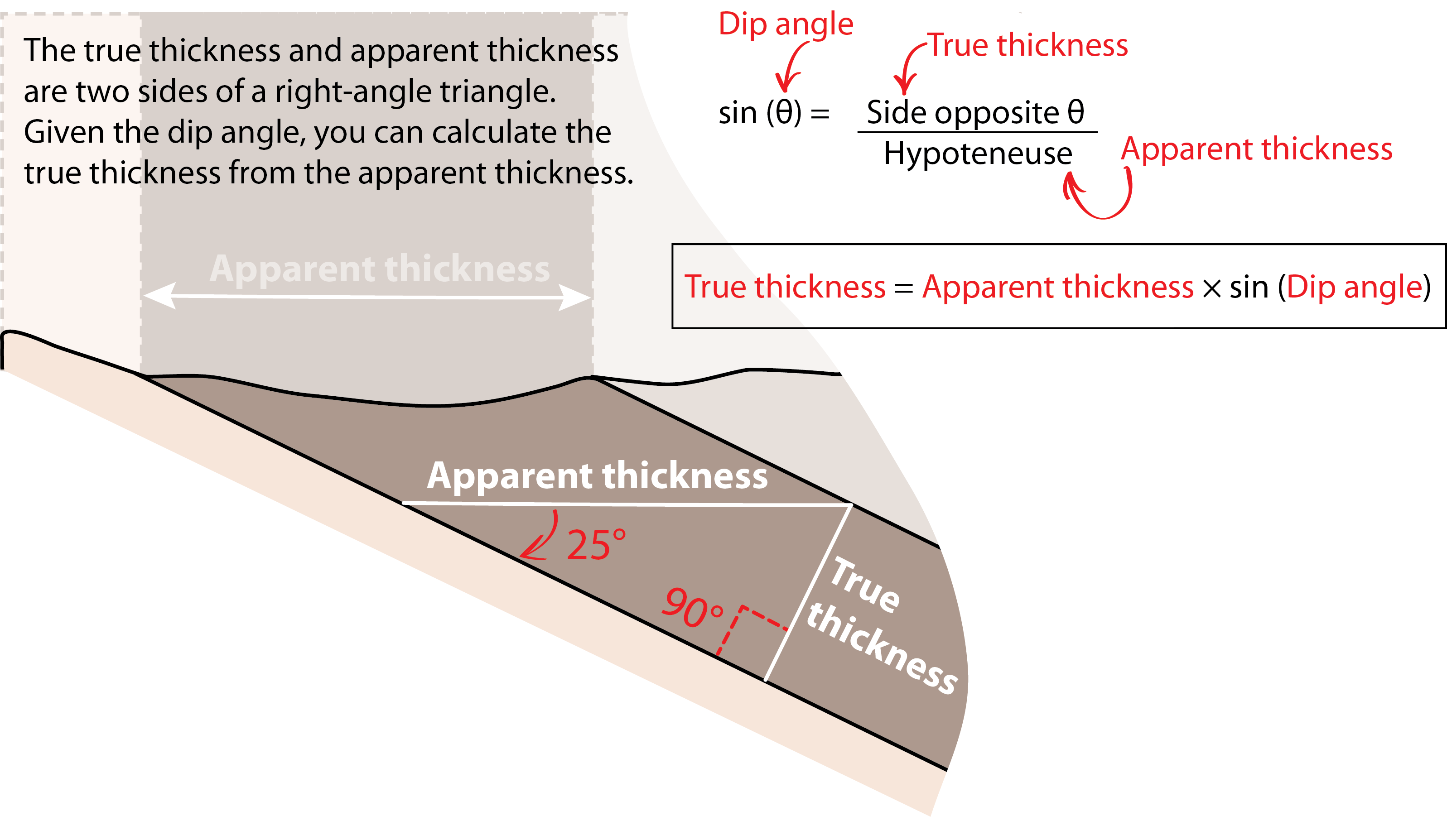
Handy Math-ternative Not Requiring a Cross-Section
(Note: For this course, use the cross-section method.) If you know the angle that the beds are dipping and the apparent thickness on the map, you can calculate the thickness of the beds using trigonometry (Figure 7.13). The true thickness is the product of the apparent thickness and the sine of the dip angle. You will need to apply the cross-section scale to your ruler measurements as with the previous method.
Special Cases: Vertical and Horizontal Beds
In situations where the beds are vertical (dip = 90˚), the thickness of the bed is equal to the distance between the upper and lower contact of the bed as measured directly on the geological map. If the beds are horizontal (dip = 0˚) and there is enough topography that both the upper and lower contacts are exposed, the thickness of the beds can be measured by calculating the difference in elevation between the upper and lower contacts with help of the contour lines.
Attributions
Adapted from:
McBeth, J., Panchuk, K., Prokopiuk, T., Hauber, L., & Lacey, S. (2020). Introductory Physical Geology Laboratory Manual, 1st Canadian Ed., Chapter 8. Geological Structures by J. McBeth, K. Panchuk, L. R. Hauber, T. C. Prokopiuk, & S. W. Lacey. CC BY-SA 4.0
Deline, B., Harris. R. & Tefend, K. (2015) Laboratory Manual for Introductory Geology, 1st Edition, Chapter 12. “Crustal Deformation” by R. Harris & B. Deline. CC BY-SA 4.0
Footnote About Why Right-Hand Rules Are Terrible
Sometimes strike and dip are reported without the dip direction specified (i.e., 045º/19º without “SE” included). When strike and dip are reported like this, there is a convention at play called the right-hand rule. Imagine holding your right hand flat on the dipping surface, with your fingers pointing downhill. If you extend your thumb straight out to the side, that’s the strike direction. Based on that rule, a bed striking at 045º could only be dipping to the SE, so it’s unnecessary to add the “SE” when you record the orientation.
The problem is, another version of the right-hand rule is that you point your thumb down-dip, and your fingers point in the strike direction. The strike and dip for a bed oriented 045º/19º SE would be reported as 225º/19º using that version. If you saw that notation and assumed the first version of the right-hand rule was in use, you would conclude the bed was dipping NW. So, if someone hires you to do geologic mapping and they want you to use the right-hand rule, make sure you find out which one. To avoid confusion, we will not use a right-hand rule for this lab, and will just have you write down the dip direction instead, like in Figure 7.7.
Note: The author feels that right-hand rules introduce a wholly unnecessary potential for error in this context. Inevitably, a right-handed person will attempt the right-hand rule while writing something down, and thus execute it with their free left hand by accident, getting it backward. If you happen to be taking an electricity and magnetism class and are right-handed, never right-hand-rule while holding a pencil, especially during an exam. Pencil down first.
