Appendix 1: Units of Measurement, Mathematical Rules, and Conversion Factors

UNITS OF MEASUREMENT IN SCIENCE

All of the various disciplines in science are concerned with the description and explanation of human-constructed and natural phenomena. The process of describing and explaining normally requires that these phenomena be quantified and measured. The purpose of this appendix is to provide you with some information on the scientific practice of making quantitative measurements in Physical Geography and Earth Science.

THE INTERNATIONAL SYSTEM OF UNITS (SI)

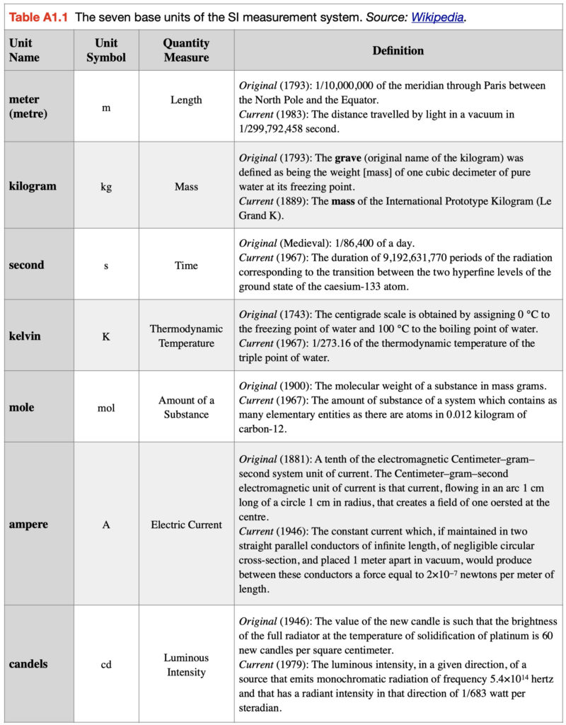
The International System of Units (abbreviated as SI) is the most commonly used system of measurement employed in science. SI is a modern adaptation of the metric system which was first introduced in France in 1799. The updated SI measurement system was originally published in 1960 as the result of a coordinated effort that started in 1948. SI has been designed to be an adapting system. As a result, new measurement units can be formulated and current measurement unit definitions can be modified through international agreement with changes in measurement science. For example, the 24th and 25th General Conferences on Weights and Measures (CGPM) in 2011 and 2014, discussed a submission to modify the definition used to describe a kilogram.

SI uses seven different base units for measurement as shown in Table A1.1. These base units are the foundation for producing other measurement units, like derived units of measurement.

Derived Measurement Units

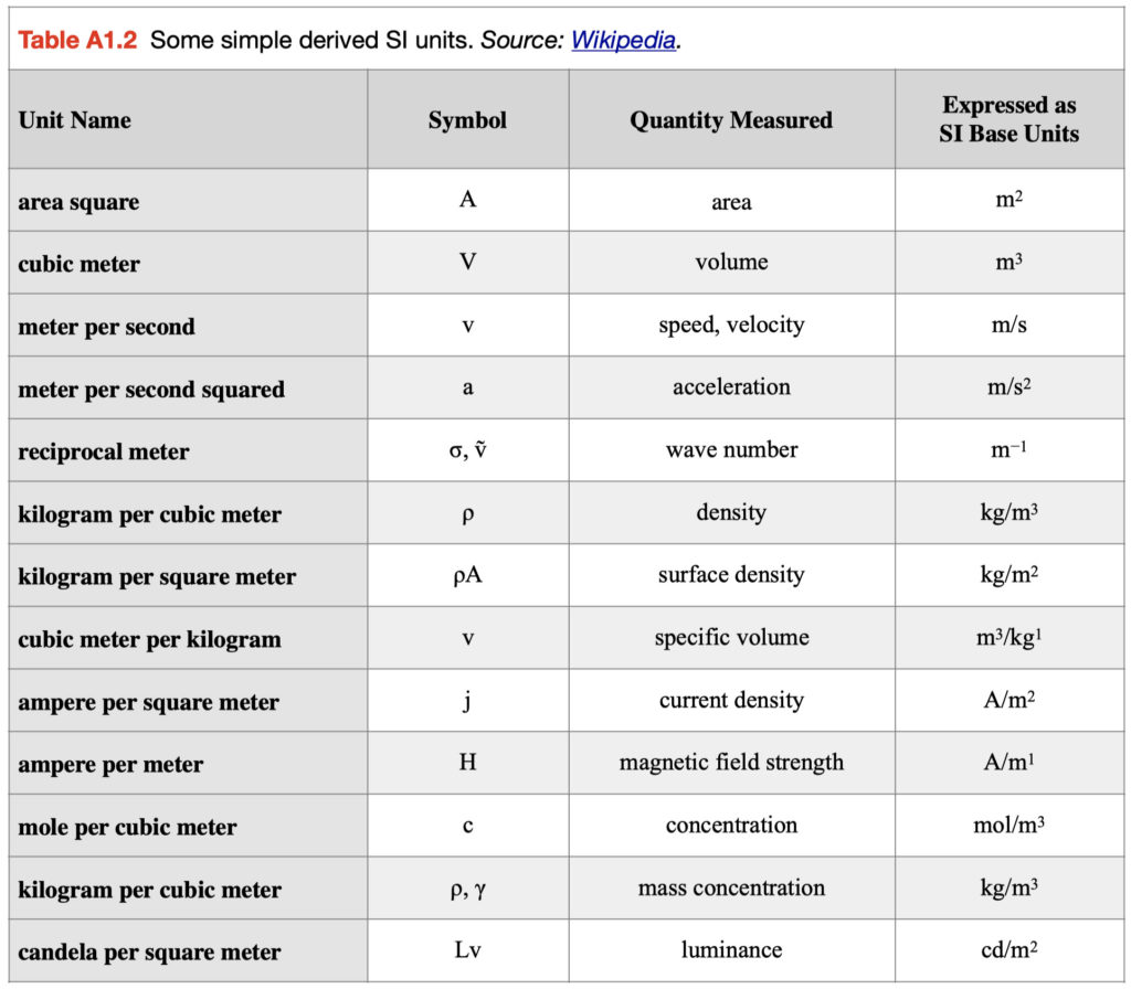
A derived unit is produced by mathematically combining base units in the SI system. A list of commonly used simple derived quantities is shown in Table A1.2. Table A1.3 shows some more derived quantities that are a bit more complex. The first unit described in this table is velocity which measures the speed of an object by combining the quantities of time and length traveled. We can measure the length traveled by the unit meter and the time it took to cover the distance traveled with the unit second. The normal convention for describing velocity is the number of meters traveled per second (meters per second) or meters traveled divided by one second (m/s or m s^-1).

Some frequently used derived measurement units have specific names and symbols to avoid the use of lengthy names and symbols formed from combining base units. For example, the SI unit for force known as a Newton (N) combines three quantities: mass, length, and time. A Newton as expressed in terms of original base units would be kilogram meter per second squared or kg m/s² or kg m s^-2. Some common derived units in this category are shown in Table A1.3 with their derivations. Note that some are derived units that come from a combination of base and other derived units.

Non-SI Units used with the SI

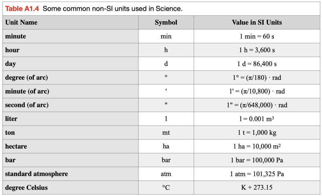
Several other measurement units not associated with the SI are used in science as well as our daily lives (Table A1.4). This includes units related to our keeping of time – minute, hour, and day; units to measure angles – degree, minute, and seconds; unit used for measuring the volume of a liquid – liter; unit used for measuring the weight of a substance – tonne; unit used for measuring area on the Earth’s surface – hectare; and units used for measuring atmospheric pressure – bar and standard atmosphere.

In the Atmospheric Sciences, temperature is often measured in °C. In the physical sciences (Astronomy, Physics, and Chemistry), the absolute or Kelvin scale of temperature is preferred. Since 0 K = -273 °C, conversion of °C to K merely requires the addition of the value 273.15. As a result, 10 °C would equal 283.15 K. Note that the Celsius scale has specifically set 0 °C (273.15 K) as the freezing temperature of pure water and 100 °C (373.15 K) as the boiling point of pure water, at sea level pressure.

Multiples and Submultiples in the SI

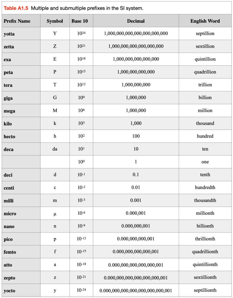
In the SI there exists a standard set of prefixes for describing the relative size of measurements (Table A1.5). These multiple or submultiple prefixes are appended to the unit to allow one to quickly identify the relative size of the measurement. For example, the unit meter (m), when multiplied by 1000 it becomes a kilometer (km) or when divided by 1000 becomes a millimeter (mm). Likewise, a Newton (N) multiplied by 1000 becomes a kilonewton (kN) and when divided by 1000 becomes a millinewton (mN). Other examples are megajoules (MJ) represents millions of joules, hectopascals (hPa) represents hundreds of Pascals, and nanometers (nm) billionths of a meter. 

MATHEMATICAL RULES

Scientific Notation

Scientific notation is a way of describing numbers that are either too large or too small to be easily written in decimal form.  It is often used by scientists to simplify arithmetic operations.

In scientific notation,  numbers are described to a base of 10 in the form:

m × 10ⁿ

where the exponent n is an integer and the coefficient m is a real number. Real numbers can be written in the form m × 10ⁿ in many ways, for example, 756  can be written as 7.56 × 10² or 75.6 × 10¹ or 756 × 10⁰.

Any number can be expressed using  base 10 exponents, for example:

700,000 (or 700 000) can be expressed as 7 x 10⁵

5,760,000,000  (or 5 760 000 000) can be expressed as 5.76 x 10⁹

0.0000777 (0.000 077 7) can be expressed as 7.77 x 10^-5

5,839,124  (5 839 124) can be expressed as 5.839124 x 10⁶ or 5.83912 x 10⁶ or 5.8391 x 10⁶ or  5.839 x 10⁶, etc. The process of showing fewer significant figures is known as rounding (see discussion below).

0.0531113 (0.053 111 3) can be expressed as 5.31113 x 10^-2 or 5.3111 x 10^-2 or 5.311 x 10^-2 or 5.31 x 10^-2,  or 5.3 x 10^-2, etc.

Basic Operations of Arithmetic

Addition (+) is a basic operation of arithmetic. The operation of addition combines two numbers  into a single number. For example,  3 + 2 = 5 or 1 + 5 = 6. The continual addition of the number 1 is the most basic form of counting. Addition obeys the mathematical Commutative Property where 7.3 + 9.8 = 9.8 + 7.3 and the Associative Property where (7.93 + 23.60) + 4.20 = 7.93 + (23.60 + 4.20).

Subtraction (-) is the inverse operation to addition. Subtraction finds the difference between two numbers. For example,  3 – 2 = 1 or 1 – 5 = -4. Subtraction does not obey Commutative Property, 7.3 – 9.8 ≠ 9.8 – 7.3, and the Associative Property, (7.93 – 23.60) – 4.20 ≠ 7.93 – (23.60 – 4.20).

Multiplication (x or · or *) is another basic operation of arithmetic. Multiplication combines two numbers (multiplier and the multiplicand) into a single number, called the product. Multiplication can be explained as  repeated addition when numbers are integers. For example, 3 x 4 = 4 + 4 + 4 = 12 or 3 x -4 =  -4 + -4 + -4 = -12. Multiplication obeys the mathematical Commutative Property where 2 x 4 = 4 x 2 and the Associative Property where (2 x 4) x 6 = 6 x (4 x 2). When using both addition and multiplication in an equation, the Distributive Property 3 x (7 + 2) = (3 x 7) + (3 x 2) applies as a truth in this operation.

Division (÷ or /) is the inverse operation to multiplication. Division determines the quotient of two numbers, the dividend divided by the divisor. Division does not obey Commutative Property, 4 ÷ 2 ≠ 2 ÷ 4, the Associative Property, (8 ÷ 2) ÷ 2 ≠ 2 ÷ (2 ÷ 8), and the Distributive Property 3 ÷ (7 + 2) ≠ (3 ÷ 7) + (3 ÷ 2).

The following examples show some common mathematical equivalencies related to addition, subtraction, multiplication and division:

y = x + n  … is the same as   x = y – n

y = n x  … is the same as   x = y ÷ n

y = nx²  … is the same as  x = √(y ÷ n)

y = a + bx … is the same as   x = (y – a)/b

y = log x  … is the same as  x = 10^y

y = ln x … is the same as  x = e^yw  ≈  2.718^y

Calculations Using Scientific Notation

Addition and Subtraction 

When doing addition and subtraction with numbers in scientific notation, all numbers involved must be expressed in the same power of ten to do calculations correctly. For example:

(1.3 x 10⁷) + (4.2 x 10⁷) = (1.3 + 4.2) x 10⁷ = 5.5 x 10⁷

(7.1 x 10⁵) – (6.1 x 10²) = (7100 x 10²) – (6.1 x 10²) = 7093.9 x 10² = 7.0939 x 10⁵

Multiplication and Division

When multiplying  numbers in scientific notation, simply ADD their exponents. When dividing SUBTRACT their exponents:

10^a x 10^b = 10^a+b , for example (1.3 x 10⁷) x (4.2 x 10⁷)  = (1.3 x 4.2) x (10⁷ x 10⁷) = 5.46 x 10¹⁴

10^a ÷ 10^b = 10^a-b, for example (2.6 x 10³) ÷ (1.3 x 10⁷)  = (2.6 ÷ 1.3) x (10³ ÷ 10⁷) = 2.0 x 10^-4

Note the following:

1 ÷ 10^a = 10^-a

1 ÷ (n * 10^a) = (1 ÷ n) * (1 ÷ 10^a)

(10^a)^b = 10^a*b

Rounding

When a value is to be rounded to less digits than the total number of original digits, please do the following:

1. When the first digit dropped is less than five, the last digit retained should not be changed. For example:

5.32139 rounded to 4 digits or 3 decimal points is 5.321

515.32139 rounded to 5 digits or 2 decimal points is 515.32

2. When the first digit dropped is five or greater, the last figure retained should be increased by one unit. For example:

7.74776 rounded to  4 digits or 3 decimal points is 7.748

114.598501 rounded to 4 digits or 3 decimal points is 114.599

The rounding method shown above is known as round half up. There are other types of rounding commonly used. See this Wikipedia link (https://en.wikipedia.org/wiki/Rounding) for more information on this topic. The other types of rounding described on this web page have been created for specific numerical purposes.

Rounding should normally take place after finishing your calculations with the original values. If this is not possible, one should use at least two more digits (decimal places) than the accuracy required from the calculation.  For example, if the required accuracy is to one decimal place:

(a) Values not rounded in the original calculation:

2.22526 + 4.50000 + 1.34453 = 8.06979, rounded to one decimal place is 8.1

(b) Values  rounded to three decimal places before the calculation (two more decimal places of accuracy than required in the answer):

2.225 + 4.500 + 1.345 = 8.070, rounded to one decimal place is 8.1 (required accuracy).

(c) Values rounded to one decimal place prior to the calculation:

2.2 + 4.5 + 1.3 = 8.0,  this procedure results in a loss of accuracy compared to the results in (a) and (b).

CONVERSION FACTORS

The following list provides some conversion factors that you may find useful relative to the study of Physical Geography and Earth Science.

Distance

1 inch (in) = 2.54 centimeters (cm)

1 foot (ft) = 0.3048 meter (m)

1 statute mile (mi) = 1.6093 kilometers (km)

1 nautical mile (NM) = 1.8532 kilometers (km)

1 meter = 39.37 inches

1 meter = 3.2808 feet

1 kilometer = 0.6214 statute miles

1 statute mile = 5280 feet

Area

1 square inch = 6.4516 cm²

1 square foot = 0.0929 m²

1 square statute mile = 2.590 km²

1 square nautical mile = 3.4348 km²

1 cm² = 0.155 square inches

1 m² = 10.764 square feet

1 km² = 0.3861 square statute mile

1 km² = 0.2912 square nautical mile

1 acre = 0.405 hectares (ha)

1 hectare = 10,000 m²

1 hectare = 2.469 acres

Volume

1 cubic inch = 16.3871 cm³

1 cubic foot = 0.0283 m³

1 cm³ = 0.0610 cubic inches

1 m³ = 35.315 cubic feet

1 m³ = 1,000.0 liters

1 US gallon = 3.785 liters

1 Imperial gallon = 4.546 liters

1 US gallon = 0.833 Imperial gallons

1 Imperial gallon = 1.20 US gallons

1 liter = 0.2642 US gallons

1 liter = 0.220 Imperial gallons

1 US ounce = 29.57 milliliters

1 Imperial ounce = 28.41 milliliters

1 US ounce = 1.041 Imperial ounces

Weight

1 grain (gr) = 0.0648 grams (g)

1 ounce (oz) = 28.35 grams (g)

1 pound (lb) = 0.4536 kilograms (kg)

1 gram (g) = 0.0035 ounces

1 kilogram (kg) = 2.2046 pounds

1 short ton (t) = 2,000.0 pounds

1 short ton = 907.185 kg

1 short ton = 0.9072 metric tons (mt)

1 metric ton = 1,000.0 kg

1 metric ton = 2204.6 pounds

1 metric ton = 1.1023 short tons

Speed

1 mile per hour (mph)=1.6093kilometers per hour (km h^-1)

1 mph=0.447meters per second (m s^-1)

1 mph=0.8684knots

1 knot=1.1516mph

1 knot=0.5148m s^-1

1 knot=1.8532km h^-1

1 km h^-1 = 0.28 m s^-1

1 km h^-1 = 0.6214 mph

1 m s^-1 = 3.6 km h^-1

1 m s^-1 = 2.237 mph

Air Pressure

1 inch mercury = 33.864 millibars (mb)

1 inch mercury = 0.0345 kg cm^-2

1 mm mercury = 1.3332 mb

1 mb = 0.0295 inch mercury

1 mb = 0.7501 mm mercury

1 mb = 0.10 kilopascals (kPa)

1 mb = 100.0 Pascals (Pa)

1 kilopascal = 10.0 mb

1 mb = 0.001 kg cm^-2

1 mb = 100.0 Newtons m^-2

Radiation and Energy

1 Watt=1.0 joule per second (J s^-1)

1 Watt per m² (W m^-2) = 0.001434   calories (cal) cm^-2 min ^-1

1 megajoule per m² (MJ m^-2) = 23.9 cal cm^-2

1 British Thermal Unit (BTU) ft ^-2 h ^-1 = 3.155 W m^-2

1 BTU ft^-2 h^-1 = 0.00452 cal cm^-2 min^-1

1 W m^-2 = 0.317 BTU ft^-2 h^-1

1 cal cm^-2 = 41.84 kilojoules m^-2 (kJ m^-2)

1 cal cm^-2 min^-1 = 697.3 W m^-2

1 cal cm^-2 min^-1 = 1.0 langley min^-1 (ly min^-1)

1 cal cm^-2 min^-1 = 221.0 BTU ft^-2 h^-1

This Appendix is Licensed Under Attribution-NonCommercial-NoDerivatives 4.0 International (CC BY-NC-ND 4.0).

Updated April 4, 2021