Michael Pidwirny
LABORATORY 3: ATMOSPHERE COMPOSITION, PRESSURE, AND CIRCULATION
LEARNING GOALS
The objectives of this laboratory are to become familiar with the composition, structure, and circulation of the Earth’s atmosphere and to understand the various physical forces that control its behavior.
Upon completion of this laboratory you will be able to:
- Describe the composition of the atmosphere, including its constituents and vertical structure.
- Understand the association between horizontal pressure gradients and patterns in wind speed and direction.
- Examine the various forces that are responsible for the atmospheric motions near the Earth’s surface and upper troposphere.
- Explain why some surface patterns of pressure exist at the global scale.
COMPOSITION OF THE ATMOSPHERE
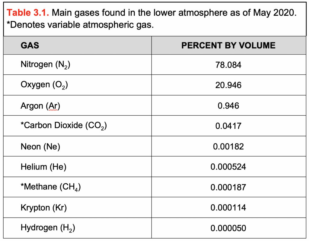
The Earth’s atmosphere (dry air) is composed of a number of different gases (Table 3.1). Most of these gases are found in the same relative proportions throughout the lower atmosphere and are referred to as the permanent gases. Mixed in with these permanent gases, are gases that vary in amount both spatially and temporally. These gases are called the variable gases.
During the last century, the proportions of the variable gases carbon dioxide and methane have been steadily increasing due to human activities. These gases play important roles in the greenhouse effect. Two other important variable gases are water vapor (H2O) and ozone (O3). Water vapor is found in the greatest concentrations near Earth’s surface and varies from 0% to 4% by volume. Ozone is found in very small amounts at 10 to 50 km above the Earth’s surface, with the maximum amount at about 25 km. Ozone helps to block some wavelengths of ultraviolet radiation from penetrating the lower atmosphere. Polar ozone holes have been detected, usually during the winter and early spring.
ATMOSPHERIC PRESSURE AND ALTITUDE
As a result of the Earth’s gravitational field, the atmosphere exerts a force on the Earth’s surface known as atmospheric pressure. It is commonly expressed in units of millibars (mb), or kilopascals (kPa), where 1 kPa = 10 mb.
The standard atmospheric pressure at the surface of the Earth is defined by international agreement as the average pressure at a latitude of 45°32′ and at a temperature of 0°C. At sea level, the standard atmospheric pressure is equal to 101.325 mb, or 1013.25 kPa. Atmospheric pressure drops rapidly with altitude above our planet’s surface (Figure 3.1).
Atmospheric pressure at the surface of the Earth varies with time, location, and changing weather conditions. It also varies with temperature, gravity, and elevation. Corrections are made to standardize the pressure data collected at all of the world’s weather stations with respect to these last three factors. These corrections make all the pressure readings on surface weather maps adjusted to sea level (regardless of weather station elevation).
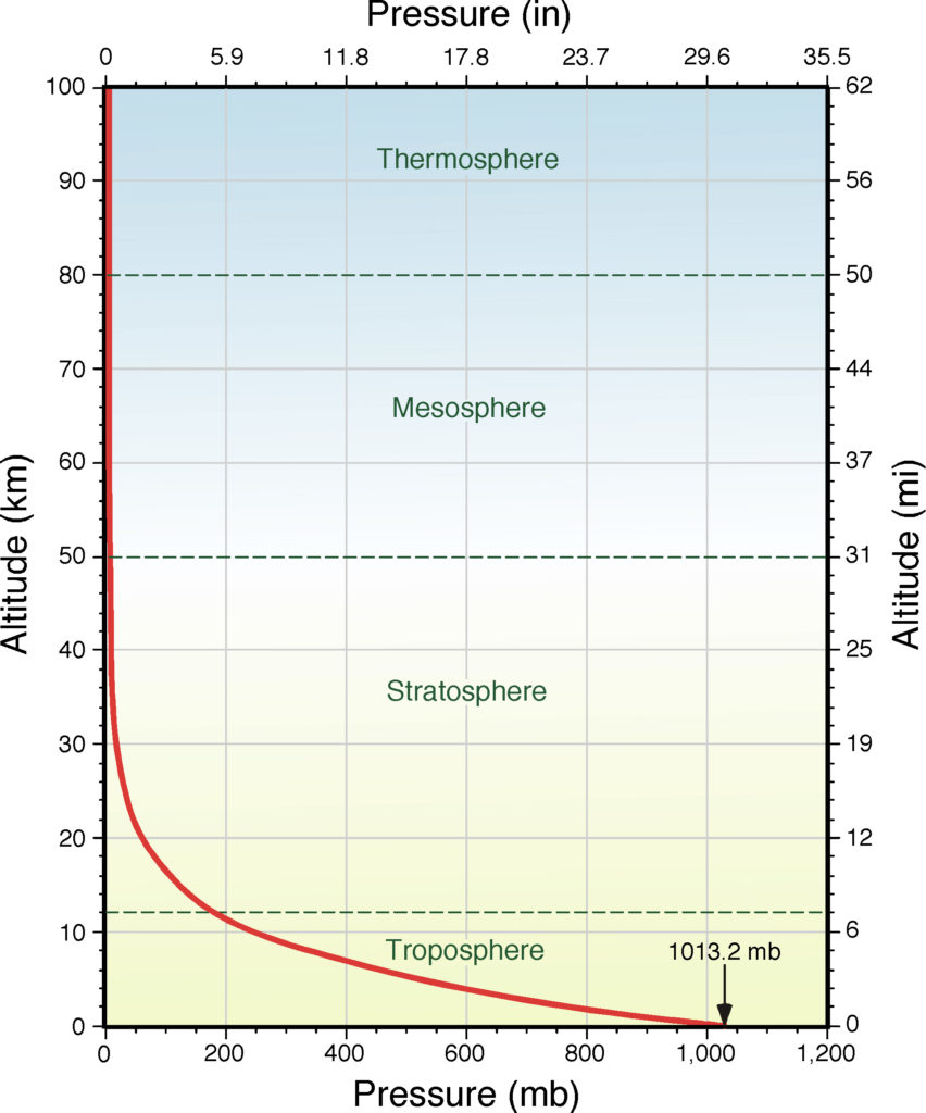
Figure 3.1. Change in average atmospheric pressure with altitude in the standard atmosphere (red line). This graph also identifies the various named layers and transition zones found in the atmosphere. Image Copyright: Michael Pidwirny.
FACTORS CONTROLLING WIND SPEED AND DIRECTION
Wind is simply air in motion. This motion can be in any direction, but in most cases the horizontal component of wind flow greatly exceeds the vertical component. The speed of wind varies from zero to ~370 km h-1 (Mt. Washington, New Hampshire, 12th April, 1934).
The direction of wind is defined as the horizontal direction from which the wind is coming, with reference to compass directions (e.g. a “north wind” comes from the North).
Pressure change over a unit distance is called the pressure gradient. A pressure gradient produces the pressure gradient force (PGF), which is the primary force influencing the speed of movement of wind. Air tries to move from areas of high pressure to areas of low pressure, usually at speeds determined by the horizontal pressure gradient.
On weather maps showing sea-level pressure, isobars show the pressure distribution; normally these are drawn at fixed 4 millibar intervals (e.g. 996 mb, 1000 mb, 1004 mb, etc.). If the isobars are closely spaced, we can expect the pressure gradient force to be great, and wind speed to be high (see Figure 3.2). In areas where the isobars are widely spaced apart, the pressure gradient is low and light winds normally exist. Further, the direction of the pressure gradient force is always perpendicular to the isobars, as indicated in the figure:
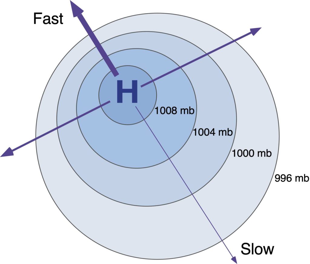
Figure 3.2. Hypothetical pressure map showing a high pressure centre (anticyclone). Isobar values are in millibars. The strength and direction of the pressure gradient force corresponds to arrow thickness and direction. Image Copyright: Michael Pidwirny.
The rotation of the Earth creates the Coriolis effect, which acts upon wind (and other objects in motion) in predictable ways. Instead of wind blowing directly from high to low pressure, the rotation of the Earth causes wind to be deflected off course. In the Northern Hemisphere, wind is deflected to the right of its path, while in the Southern Hemisphere it is deflected to the left. The strength of the Coriolis Effect (CE) is given by the following equation:
Coriolis Effect (CE) = 2 Ω sin Θ u
where: u = wind speed (m s-1), Ω = Earth rotation rate = 7.29 x 10⁻⁵ (s-1), and Θ = latitude (degrees).
What this tells us is that the magnitude of the Coriolis effect varies directly with two different things: wind speed and the latitude of the moving object (assuming a constant rotation rate for the Earth). From this we can conclude: (1) Coriolis effect is absent at the Equator and its strength increases as one approaches the poles; and (2) Coriolis effect increases with wind speed.
Air under the influence of both the pressure gradient force and the Coriolis effect tends to move parallel to isobars in conditions where friction is very low (typically, greater than 1 to 2 km above the surface of the Earth) and isobars are straight. Winds of this type are usually called geostrophic winds. Geostrophic winds come about because pressure gradient force and the Coriolis effect come into balance (Figure 3.3). Buy Ballot's Law states that when you stand with your back to a geostrophic wind in the Northern Hemisphere the area of lower pressure will be to your left and the higher pressure to your right. The opposite is true for the Southern Hemisphere.
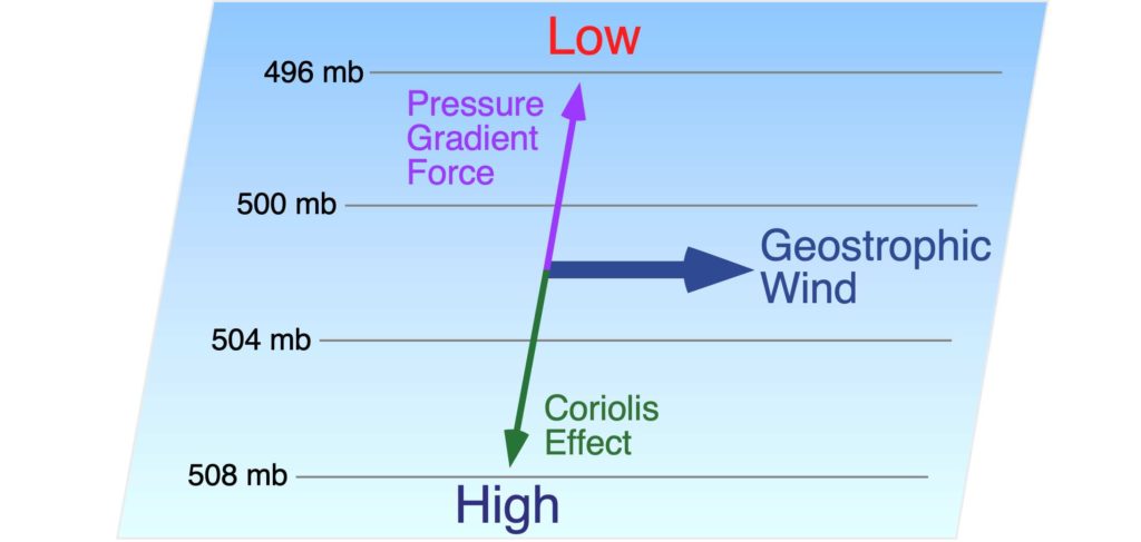
Figure 3.3. In the upper atmosphere, the effects of friction are nonexistent and this results in a balance between pressure gradient force and the Coriolis effect. This balance causes the resulting upper air winds to flow parallel to the isobars. These upper air winds are known as geostrophic winds. Image Copyright: Michael Pidwirny.
In many cases, winds flow around the curved isobars of a high pressure centre (anticyclone) or low pressure centre (cyclone). Above the level of friction these winds are called gradient winds. Gradient winds are slightly more complex than geostrophic winds because they include the action of centripetal force, which is always directed toward the centre of rotation. Figure 3.4 describes the forces that produce gradient winds around high and low pressure centres. Around a low, the gradient wind consists of the pressure gradient force and centripetal force acting toward the centre of rotation, while the Coriolis effect acts away from the centre of the low. In a high pressure centre, the Coriolis and centripetal forces are directed toward the centre of the high, while the pressure gradient force is directed outward.
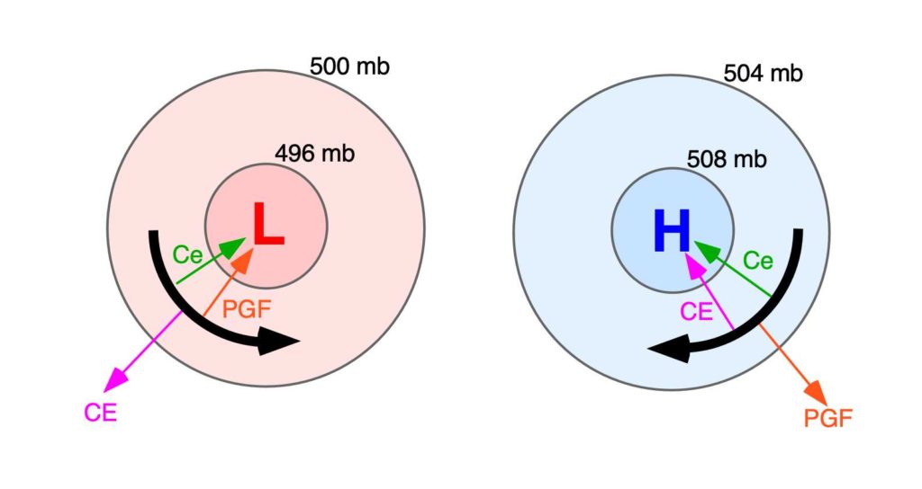
Figure 3.4. The balance of forces that create a gradient wind in the Northern Hemisphere (PGF = pressure gradient force; CE = Coriolis effect; and Ce = centripetal force). In this diagram, CE = Ce + PGF for the low pressure center (cyclone), and PGF = CE + Ce for the high pressure center (anticyclone). Image Copyright: Michael Pidwirny.
SURFACE WINDS
Surface winds on a weather map do not travel exactly parallel to the isobars. Instead, they tend to cross the isobars at an angle varying from 10 to 45°. Close to the Earth’s surface, friction reduces the wind speed, which in turn reduces the Coriolis effect. As a result, the reduced Coriolis effect no longer balances the pressure gradient force, and the wind blows across the isobars toward the area with lower pressure (Figure 3.5). The pressure gradient force is now balanced by the sum of the frictional force and the Coriolis effect.
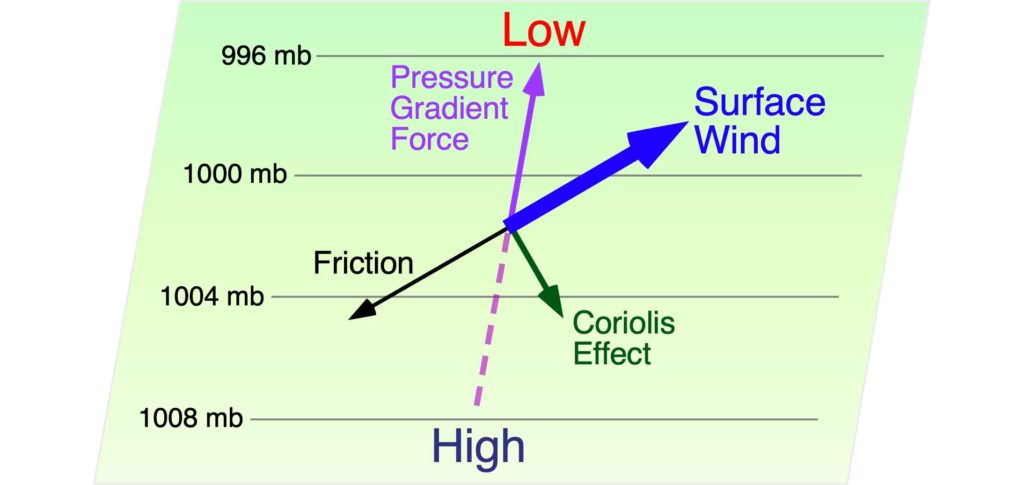
Figure 3.5. Winds near the Earth’s surface are influenced by pressure gradient force, the Coriolis effect, and surface friction. Image Copyright: Michael Pidwirny.
As a result, we find surface winds blowing counter-clockwise and inward into a surface low, and clockwise and out of a surface high in the Northern Hemisphere (Figure 3.6). In the Southern Hemisphere, the Coriolis effect acts to the left rather than the right. This causes the winds of the Southern Hemisphere to blow clockwise and inward around surface lows, and counter-clockwise and outward around surface highs.
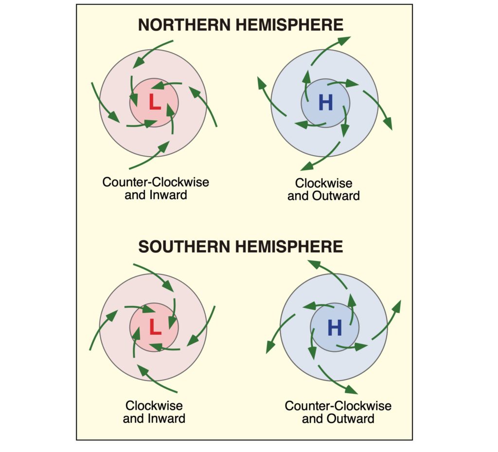
Figure 3.6. The direction of surface winds around high and low pressure systems. Image Copyright: Michael Pidwirny.
THERMAL CIRCULATION SYSTEMS
As discussed earlier, winds blow because of variations in atmospheric pressure. Pressure gradients may develop on a local to a global scale because of differences in the heating and cooling of the Earth’s surface. Heating and cooling cycles that develop daily or annually can create several common local or regional thermal wind systems. The basic circulation system that develops is described in Figure 3.7.
In this first diagram (A – Figure 3.7), there is no horizontal temperature or pressure gradient and therefore no wind. Atmospheric pressure decreases with altitude as depicted by the drawn isobars (1000 to 980 mb). In the second diagram (B – Figure 3.7), the potential for solar heating is added which creates contrasting surface areas of temperature and atmospheric pressure. The area to the right receives more solar radiation and the air begins to warm from heat energy transferred from the ground through conduction and convection. The vertical distance between the isobars becomes greater as the air rises. To the far left, less radiation is received because of the presence of cloud, and this area becomes relatively cooler than the area to the right. In the upper atmosphere, a pressure gradient begins to form because of the rising air and upward spreading of the isobars. The air then begins to flow in the upper atmosphere from high pressure to low pressure.
Diagram C (Figure 3.7) shows a fully developed thermal circulation system. Beneath the upper atmosphere high, is a thermal low-pressure center created from the heating of the ground surface. Below the upper atmosphere low, is a thermal high created by the relatively cooler air temperatures and the descending air from above. Surface air temperatures are cooler here because of the obstruction of shortwave radiation absorption at the Earth’s surface by the cloud. At the surface, the wind blows from high to low pressure. Once at the low, the wind rises up to the upper air high-pressure system because of thermal buoyancy and outflow in the upper atmosphere. From the upper high, the air travels to the upper air low, and then back down to the surface high to complete the circulation cell. Note that the thermal circulation cell is a closed system that redistributes air from areas that have a surplus to areas that have a deficit (in terms of air pressure). This circulation cell is driven by the greater heating of the surface air in the right side of the diagram.
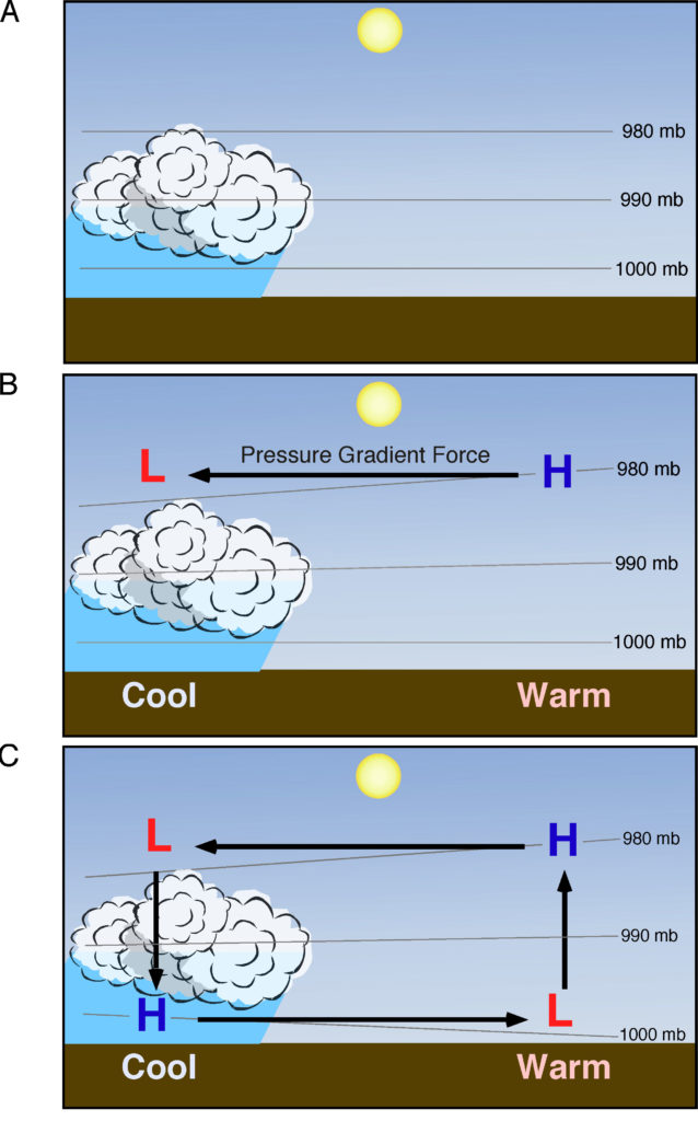
Figure 3.7. The formation of a thermal circulation system. This process begins with the unequal heating of the Earth’s surface and lower atmosphere (A). The unequal heating causes the isobars over the area being heated to spread apart because of convection and air expansion. This process also initiates the horizontal flow of air in the upper atmosphere (B). Air flow patterns then begin in the vertical and near the ground surface completing the circulation system (C). Image Copyright: Michael Pidwirny.
LABORATORY 3 QUESTIONS
QUESTION 1
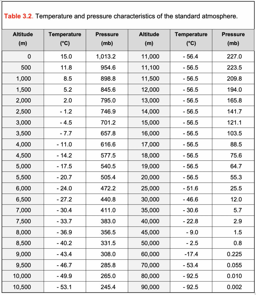
Using the information in Table 3.2, interpolate the atmospheric pressure (in mb) for each of the following locations. Round off your answers to one decimal place.
Example: Dilworth Mountain Peak, Kelowna, British Columbia, Canada: 636 m.
Step 1: Find the pressure for known altitudes either side of the elevation of interest:
Pressure at 500 m = 954.6 mb
Pressure at 1000 m = 898.8 mb
Step 2: Calculate the per meter rate of pressure change between the two known altitudes:
954.6 – 898.8 = 55.8 mb
1000 – 500 = 500 m
55.8 /500 = 0.1116 mb m-1 (rate pressure drops with an increase in altitude)
Step 3: Find the height difference between the elevation of interest and the lower boundary of the known values:
636 – 500 = 136 m
Step 4: Calculate the pressure at the location using the values calculated in Steps 2 and 3:
Pressure at 636 m = 954.6 – (136 * 0.1116) = 939.4 mb
1.1) What is the approximate atmospheric pressure of Victoria, British Columbia, Canada 23 meters above sea level in millibars?
1.2) What is the approximate atmospheric pressure of Kelowna, Canada 344 meters above sea level in millibars?
1.3) What is the approximate atmospheric pressure of Mt. Sidley, Antarctica 4181 meters above sea level in millibars?
1.4) What is the approximate atmospheric pressure of Mt. Everest, Nepal 8848 meters above sea level in millibars?
1.5) What is the approximate atmospheric pressure of Death Valley, U.S.A.: -86 meters below sea level in millibars?
1.6) What is the approximate atmospheric pressure of Big White Peak, Canada 2319 meters above sea level in millibars?
1.7) What is the approximate atmospheric pressure of Vail Ski Resort Peak, Colorado, USA 3527 meters above sea level in millibars?
QUESTION 2
Answer the following questions related to the structure and the chemical composition of the atmosphere.
2.1) Excluding the thermosphere, what atmospheric layer contains the warmest air temperatures? How are these temperatures affected by the ground surface of our planet?
2.2) Why are warm temperatures also found in the stratosphere? What process is creating the heat energy found here?
2.3) Using the data in Table 3.2, and information in Figure 3.1 derive the average lapse rate for the troposphere.
Average lapse rate = __ °C per km.
Show your calculations:
2.4) The following web address takes you to NOAA’s Global Monitoring Laboratory for atmospheric carbon dioxide (CO2).
https://www.esrl.noaa.gov/gmd/ccgg/trends/
Using the Mauna Loa, Hawaii data, select the tab “Interactive Plots”. On the top graph, turn off the display for CO2. This should leave you with just a blue trend line (see image below).
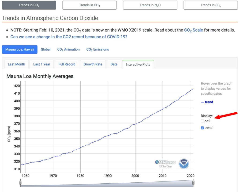
2.4a) Select the blue trend line and determine the quantity of carbon dioxide (ppm) on January, 1960. Record your answer to 2 decimal points.
2.4b) Select the blue trend line and determine the quantity of carbon dioxide (ppm) on December, 1969. Record your answer to 2 decimal points.
2.4c) What was the net increase in atmospheric carbon dioxide from January, 1960 to December, 1969 in ppm (record your answer to 2 decimal points)?
2.4d) Select the blue trend line and determine the quantity of carbon dioxide (ppm) on January, 2010. Record your answer to 2 decimal points.
2.4e) Select the blue trend line and determine the quantity of carbon dioxide (ppm) on December, 2019. Record your answer to 2 decimal points.
2.4f) What was the net increase in atmospheric carbon dioxide from January, 2010 to December, 2019 in ppm (record your answer to 2 decimal points)?
2.4g) From your calculations, would you conclude the rate of increase of atmospheric carbon dioxide from 1960 is
A the same.
B now about two times greater.
C now about three times greater.
QUESTION 3
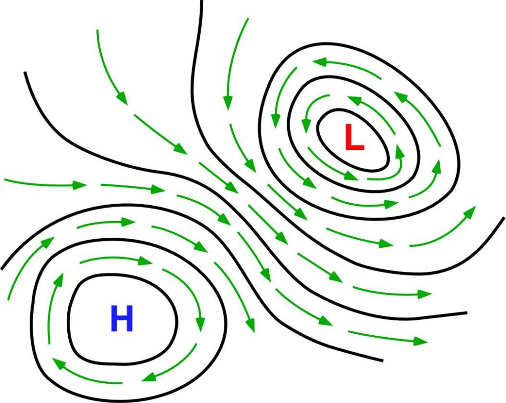
3.1) Which of the following circulation patterns represents a low pressure system in the Southern Hemisphere?
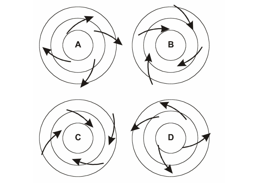
3.2) Which of the following circulation patterns represents a high pressure system in the Southern Hemisphere?
3.3) Which of the following circulation patterns represents a high pressure system in the Northern Hemisphere?
QUESTION 4
The next four questions will show you wind patterns at the Earth’s surface and in the upper atmosphere. Also, determine if the patterns are from the Northern Hemisphere of the Southern Hemisphere.
4.1) The wind pattern shown in the following map is
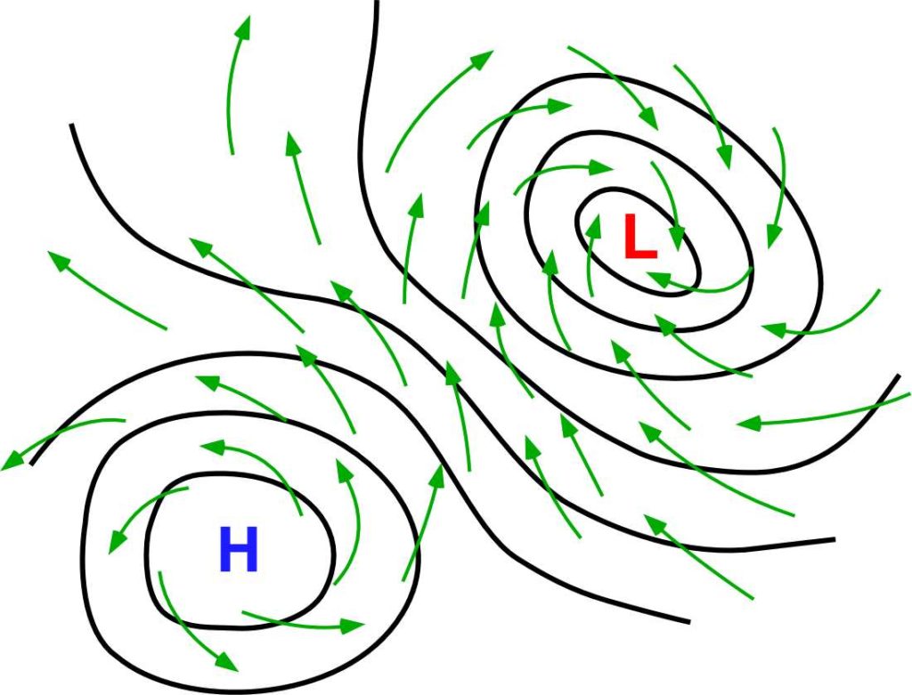
A surface winds in the Northern Hemisphere.
B surface winds in the Southern Hemisphere.
C upper air winds in the Northern Hemisphere.
D upper air winds in the Southern Hemisphere.
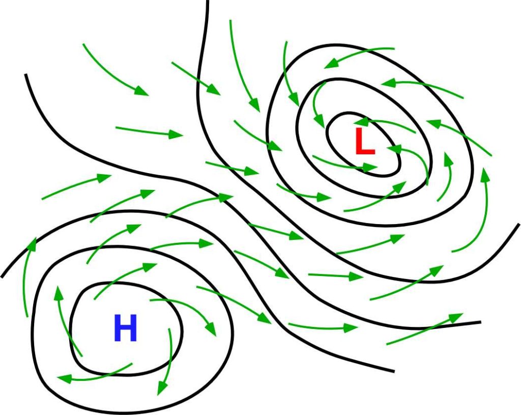
4.2) The wind pattern shown in the following map is
A surface winds in the Northern Hemisphere.
B surface winds in the Southern Hemisphere.
C upper air winds in the Northern Hemisphere.
D upper air winds in the Southern Hemisphere.
4.3) The wind pattern shown in the following map is
A surface winds in the Northern Hemisphere.
B surface winds in the Southern Hemisphere.
C upper air winds in the Northern Hemisphere.
D upper air winds in the Southern Hemisphere.
4.4) The wind pattern shown in the following map is
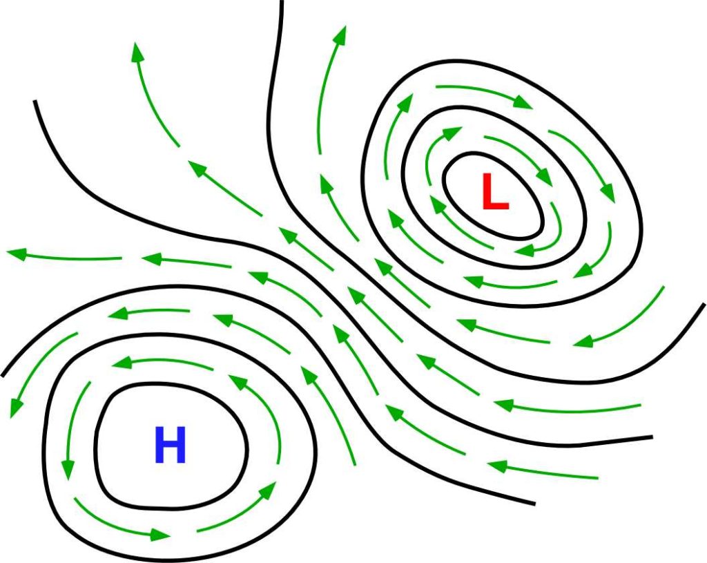
A surface winds in the Northern Hemisphere.
B surface winds in the Southern Hemisphere.
C upper air winds in the Northern Hemisphere.
D upper air winds in the Southern Hemisphere.
QUESTION 5
The following map shows sea level pressure over a region. This region is dominated by a low and high pressure system. Isobars are drawn around these pressure centers at a 4 millibar (mb) interval.
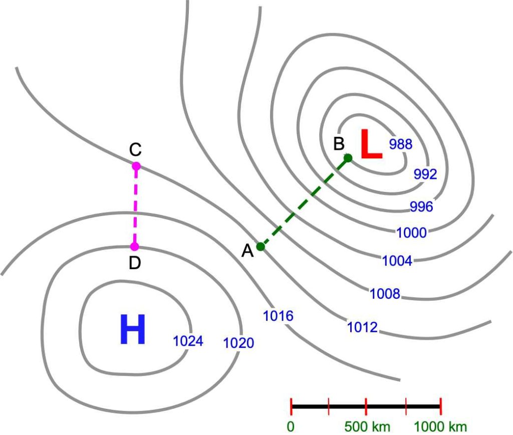
Calculate the pressure gradient (difference in pressure between stations divided by the distance between them) between A – B and C – D. Express the pressure gradient to 3 decimal places, in units of mb km-1 (millibars per kilometer). Answer the following questions.
5.1) The calculated pressure gradient for A – B which has a distance of 750 kilometers between points is
5.2) The calculated pressure gradient for C – D which has a distance of 500 kilometers between points is
5.3) How much faster are the winds in A – B relative to C – D?
A 0.5 times.
B 2 times.
C 3 times.
D 4 times.
Here is the sea level pressure map again with some slight modifications. Drawn on it are three locations – X, Y, and Z. Answer the following questions.
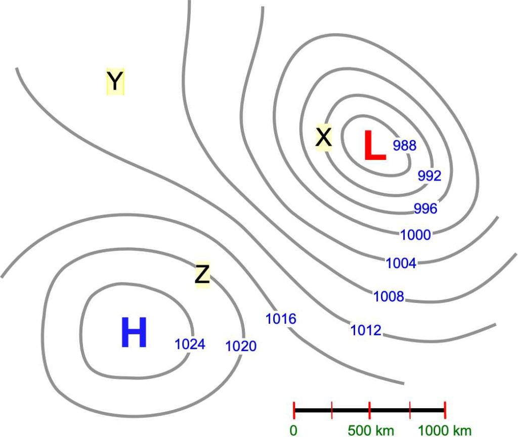
5.4) Which location would have the fastest wind speed?
A X
B Y
C Z
5.5) Which location would have the slowest wind speed?
A X
B Y
C Z
QUESTION 6
Use the following web link to go to Climate Reanalyzer, Monthly Reanalysis Maps.
http://climatereanalyzer.org/reanalysis/monthly_maps/
Create a global map showing annual average mean sea level pressure for the 30-year period 1981-2010 with the following inputs.
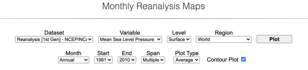
Answer the following questions.
6.1) Atmospheric pressure along the equator averages about
A 990 mb.
B 1000 mb.
C 1010 mb
D 1020 mb.
6.2) The pressure patterns seen at the equator are related directly to the
A Intertropical Convergence Zone.
B Tropical Low Pressure Zone.
C Zone of Hurricane Enhancement.
D Subtropical High Pressure Zone.
6.3) The high pressure patterns located over the oceans at 30° N and S are called the
A Intertropical Convergence Zone.
B Oceanic Highs.
C Zone of Hurricane Enhancement.
D Subtropical High Pressure Zone.
6.4) In the Northern Hemisphere, the Subpolar Lows can be found in the following locations.
A Southern Alaska and around the Aleutian Islands.
B Around the tip of Greenland and over Iceland.
C Southern Canada.
D Western Europe.
6.5) Why are the Subpolar Lows so intense and continuous in the Southern Hemisphere?
Do not close your global map showing annual average mean sea level pressure. Now create a SECOND global map showing Winter (DJF – December/January/February) average mean sea level pressure for the 30-year period 1981-2010 with the following inputs. Create this map in a separate window so you can make comparisons to the annual average. January is the winter season in the Northern Hemisphere and the landmasses are cooling much more than the ocean bodies. In the Southern Hemisphere summer is occurring and the landmasses are heating up more than the ocean bodies.
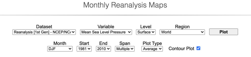
http://climatereanalyzer.org/reanalysis/monthly_maps/
Answer the following questions.
6.6) How does the location of area of low pressure (ITCZ) along the equator change from the annual plot to the Winter plot?
A It moves south mainly below the equator.
B It moves north mainly above the equator.
6.7) Explain what happened in question 6.6.
6.8) How does the subtropical high pressure zone in the Northern Hemisphere change from the annual plot to the Winter plot?
A It intensifies and becomes more prominent over the continents that are now much cooler in temperature.
B It weakens and becomes less prominent over the continents that are now much cooler in temperature.
6.9) Explain what happened in question 6.8.
6.10) How does the subpolar low pressure zone in the Northern Hemisphere change from the annual plot to the January plot?
A It intensifies and becomes more prominent over the oceans.
B It weakens and becomes less prominent over the oceans.
6.11) Explain what happened in question 6.10.
Once again, do not close your global map showing annual average mean sea level pressure. Create a THIRD global map showing Summer (JJA – June/July/August) average mean sea level pressure for the 30-year period 1981-2010 with the following inputs. Create this map in a separate window so you can make comparisons to the annual average. July is the summer season in the Northern Hemisphere and the landmasses are heating up faster than the ocean bodies. In the Southern Hemisphere winter is occurring and the landmasses are cooling a lot more than the ocean bodies.
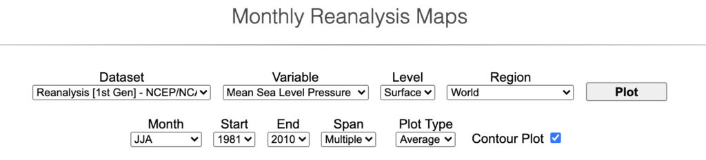
http://climatereanalyzer.org/reanalysis/monthly_maps/
Answer the following questions.
6.12) How does the location of area of low pressure (ITCZ) along the equator change from the annual plot to the Summer plot?
A It moves south mainly below the equator.
B It moves north mainly above the equator.
6.13) Explain what happened in question 6.12.
6.14) How does the subtropical high pressure zone in the Northern Hemisphere change from the annual plot to the Summer plot?
A It intensifies and becomes more prominent over the continents that are now much warmer in temperature.
B It weakens and becomes less prominent over the continents that are now much warmer in temperature.
6.15) Explain what happened in question 6.14.
6.16) How does the subpolar low pressure zone in the Northern Hemisphere change from the annual plot to the Summer plot?
A It intensifies and becomes more prominent over the oceans.
B It weakens and becomes less prominent over the oceans.
6.17) Explain what happened in question 6.16.
IMAGE CREDITS
Figure 3.1: Image Copyright Michael Pidwirny.
Figure 3.2: Image Copyright Michael Pidwirny.
Figure 3.3: Image Copyright Michael Pidwirny.
Figure 3.4: Image Copyright Michael Pidwirny.
Figure 3.5: Image Copyright Michael Pidwirny.
Figure 3.6: Image Copyright Michael Pidwirny.
Figure 3.7: Image Copyright Michael Pidwirny.
QUESTION ANSWER SHEET
This Laboratory Exercise is Licensed Under Attribution-NonCommercial-NoDerivatives 4.0 International (CC BY-NC-ND 4.0).
Updated April 5, 2021
Common gas found in the atmosphere. Carbon dioxide can selectively absorb radiation in the longwave band. This absorption causes the greenhouse effect. The concentration of this gas has been steadily increasing in the atmosphere over the last three centuries due to the burning of fossil fuels, deforestation, and land-use change. Some scientists believe higher concentrations of carbon dioxide and other greenhouse gases will result in an enhancement of the greenhouse effect and global warming. The chemical formula for carbon dioxide is CO2.
Methane is very strong greenhouse gas found in our planet’s atmosphere. Methane concentrations in the atmosphere have increased by more than 140% since 1750. The primary sources for the additional methane added to the atmosphere (in order of importance) are: rice cultivation, domestic grazing animals, termites, landfills, coal mining, and oil and gas extraction. Chemical formula for methane is CH4.
The greenhouse effect causes the atmosphere to trap more heat energy at the Earth's surface and within the atmosphere by absorbing and reemitting longwave radiation. Of the longwave energy emitted back to space, 90% is intercepted and absorbed by greenhouse gases. Without the greenhouse effect the Earth's annual mean global temperature would be -18°C (-0.4°F), rather than the present 15°C (59°F). In the last few centuries, the activities of humans have directly or indirectly caused the concentration of the major atmospheric greenhouse gases to increase. Scientists predict that this increase may enhance the greenhouse effect making the planet warmer. Some experts estimate that the Earth's annual mean global temperature has already increased by 0.3 to 0.6°C (0.5 to 1.0°F), since the beginning of this century, because of this enhancement.
Triatomic oxygen that exists in the Earth's atmosphere as a gas. Ozone is highest in concentration in the stratosphere (10 to 50 kilometers (6.2 to 31.1 miles) above the Earth's surface) where it absorbs the Sun's ultraviolet radiation. Stratospheric ozone is produced naturally and helps to protect life from the harmful effects of solar ultraviolet radiation. Over the last few decades levels of stratospheric ozone have been declining globally, especially in Antarctica. Scientists have determined that chlorine molecules released from the decomposition of chlorofluorocarbons (CFCs) are primarily responsible for ozone destruction in the stratosphere. It is also abundant near the Earth's surface (troposphere) in highly polluted urban centers. In these areas, it forms as a by product of photochemical smog, and is hazardous to human health.
The weight of the atmosphere on a surface. At sea level, the average atmospheric pressure is 1013.25 millibars (29.92 inches of mercury). Atmospheric pressure can be measured by a device called a barometer.
A unit measurements for quantifying force. Used to measure atmospheric pressure. Equivalent to 1,000 dynes per square centimeter.
An International System of Units unit of measurement for quantifying force. Used to measure atmospheric pressure. Equal to one newton over an area of one square meter. Equivalent to 10,000 dynes per square centimeter or 1,000 Pascals.
A pressure of 101325 pascals (Pa) or 101.325 kilopascals (kPa) or 1013.25 millibars (mb).
A mass of air moving horizontally and/or vertically.
The force due to spatial differences in atmospheric pressure. Usually expressed in millibars or kilopascals per unit distance measured in meters or kilometers. This force is mainly responsible for the development of wind.
Is a line (isoline) on a map joining points of equal atmospheric pressure.
An apparent force due to the Earth rotation and the spherical shape of our planet’s surface. This apparent force causes moving objects to be deflected to the right in the Northern Hemisphere and to the left in the Southern Hemisphere. Coriolis effect does not exist on the equator. This force is responsible for the direction of flow in meteorological phenomena like mid-latitude cyclones, hurricanes, and anticyclones. Coriolis effect also has a role in the formation of the Ekman spiral and Ekman transport in ocean bodies.
Describes the spatial relationship between wind direction and atmospheric pressure distribution. In the Northern Hemisphere it states: for a person who has his back to the wind, the high pressure system would on their right and the low pressure system on their left. In the Southern Hemisphere it states: for a person who has his back to the wind, the high pressure system would on their right and the low pressure system on their left. First stated in 1857 by Dutch meteorologist C.H.D. Buys Ballot.
A horizontal wind in the upper atmosphere that moves parallel to curved isobars. Results from a balance between pressure gradient force, Coriolis effect, and centripetal force.
Force required to keep an object moving in a circular pattern around a center of rotation. This force is directed towards the center of rotation. Common in meteorological phenomena like tornadoes and hurricanes.
The resistance that occurs between the contact surfaces of two bodies in motion.
Force acting on wind near the Earth's surface because of frictional roughness. This force causes a reduction in wind speed.
