Michael Pidwirny
LABORATORY 2: HEAT AND TEMPERATURE IN THE ATMOSPHERE
LEARNING GOALS
The objectives of this laboratory are to familiarize you with the concept of temperature and its measurement, and to explain why surface and near-surface air temperatures vary over time and space.
Upon completion of this laboratory you will be able to:
- Describe the various scales used to measure temperature.
- Understand the reasons why air temperature varies vertically at and near the Earth’s surface.
- Explain why air temperature varies spatially and temporally across our planet’s surface.
- Comprehend how land and ocean surfaces influence air temperature in different ways.
TEMPERATURE AND HEAT
Temperature is the condition that determines the flow of heat (a form of energy) from one body to another body. In nature, heat always flows from a warm body to a cold body. If there is no flow of heat between bodies they will have the same temperature. If one body receives heat energy from another body, the first body must be of lower temperature. Temperature can also be defined as the measure of the average speed of atoms and molecules. The higher the temperature, the faster these particles of matter move. At a temperature of -273.15°Celsius (absolute zero) all atomic motion stops.
Three temperature scales are in common use: Fahrenheit (°F), Celsius (°C), and Kelvin (K). The scientific world has adopted the Celsius scale for most uses; this scale is based on the freezing point (0°C) and boiling point (100°C) of water under standard conditions. The Kelvin scale is most appropriate in some equations and laws (e.g. the radiation laws).
The conversion equations are:
T(°C)= 5/9 x (T(°F) – 32)
T(°C)= T(K) – 273
T(°F) = (9/5 x T(°C)) + 32
T(K)= T(°C) + 273
THERMOMETERS
Thermometers are instruments that measure temperature. The first thermometer was introduced in the early 1600s using the expansion of air to show changes in ambient temperature. This instrument, however, was subject to many sources of error. Other types of instruments followed, trying to gain greater accuracy of measurement. In 1714, Gabriel Daniel Fahrenheit introduced the mercury thermometer and his famous scale of measurement. Fahrenheit’s measurement scale was based on the fact that the boiling and freezing point of pure water is constant. For zero on his scale, he selected the lowest temperature he could achieve by a mixture of ice and common salt. For the other fixed point on his scale, he used body temperature and assigned it the value of 96.
In normal meteorological practice, digital, mercury, and alcohol thermometers are used by weather services such as the Meteorological Service of Canada to measure surface air temperature. The highest and lowest temperatures in a particular period are read from self-registering maximum thermometer and minimum thermometer that are placed in a ventilated Stevenson screen designed to protect these instruments from direct solar radiation. Maximum daily surface air temperatures are usually measured by a mercury thermometer. Alcohol thermometers are used to measure surface air temperature minimums because mercury freezes below -39°C.
VERTICAL DISTRIBUTION OF AIR TEMPERATURE
While pressure always decreases with altitude, the vertical pattern of atmospheric temperature is quite different. A lapse rate is simply the mathematical expression of the temperature change with height; mathematically, this is equal to:
lapse rate = ΔT/Δz
where T is air temperature (°C), z is altitude (in meters), and Δ (delta) simply means “change in”.
Figure 2.1 shows the Earth’s standard atmosphere, which can be thought of as the average conditions for the planet. Note that average air temperature is about 15°C at the surface and decreases with altitude until a transition zone called the tropopause is reached, where the temperature remains fairly uniform. Actual rates of tropospheric temperature change vary with altitude, location, and time of year. Each of these rates is referred to as an environmental lapse rate (ELR). Sometimes close to the Earth’s surface temperatures warm up with altitude. This condition, known as a temperature inversion, can be produced by the overnight cooling of the near-surface air by longwave radiation emission that is directed towards space.
The tropopause is typically at about 18 km near the Equator, and only about 8 km at the poles. The layer between the surface and the tropopause is known as the troposphere. Most of our planet’s weather occurs in this layer.
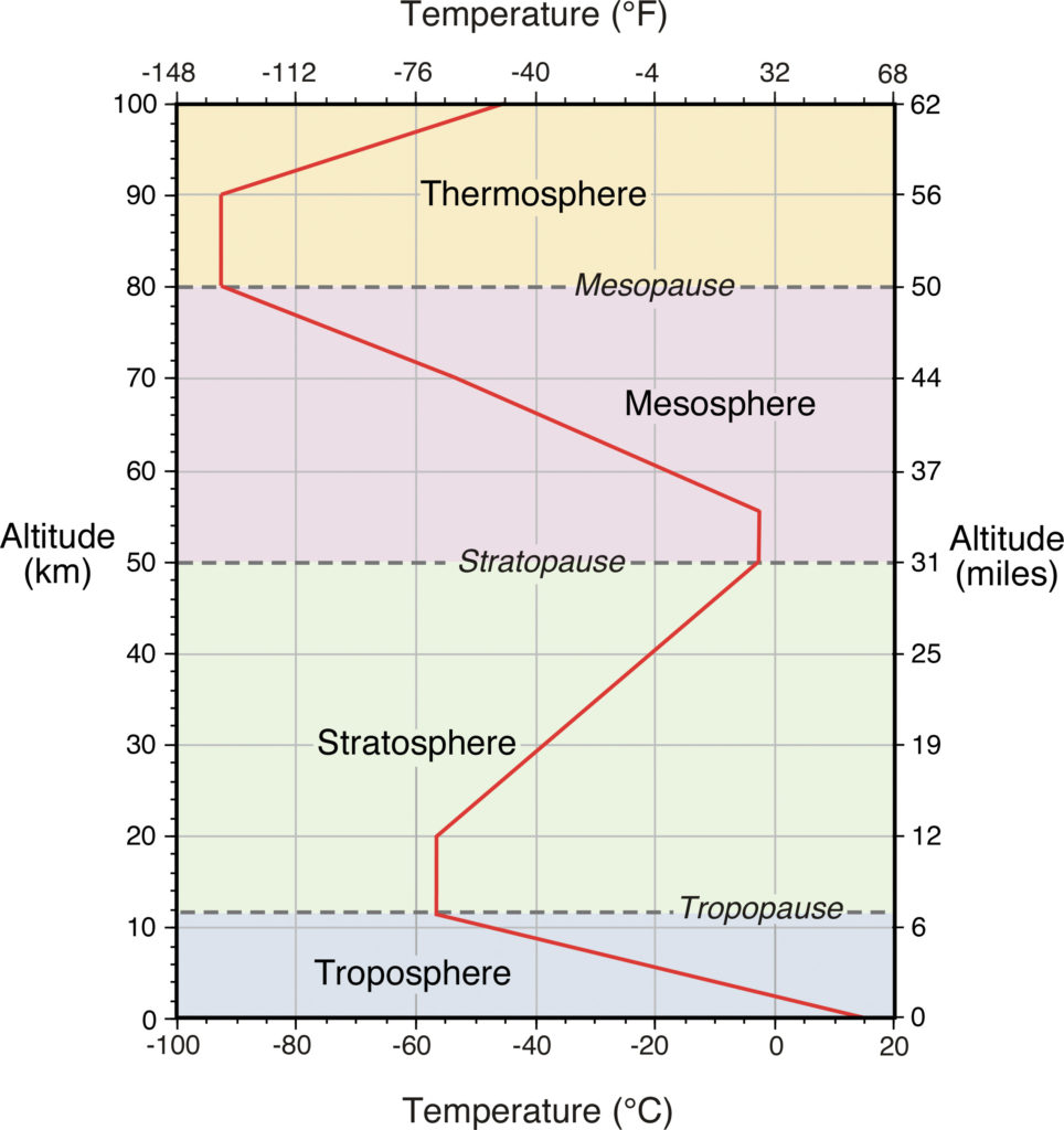
Figure 2.1. Change in average atmospheric temperature with altitude in the standard atmosphere. This graph also identifies the various named layers and transition zones found in the atmosphere. Image Copyright: Michael Pidwirny.
Above the troposphere, to an elevation of about 50 km, there is the stratosphere. Here, atmospheric temperature increases because of the absorption of solar ultraviolet radiation by ozone. The stratosphere is capped by the stratopause and the mesosphere lies above at about 50 to 80 km. In the mesosphere, temperatures decrease with height, and we find the coldest temperatures in the atmosphere (about -90°C) at the upper boundary of this layer (the mesopause). The highest temperatures (>1000°C), are reached in the thermosphere (85 km to the atmosphere’s outermost fringe).
DAILY AND SEASONAL CHANGES IN SURFACE AIR TEMPERATURE
Figure 2.2 shows a simple time series graph of insolation and surface air temperature over a 24-hour period. This data represents a typical cloudless summer day in the middle latitudes. Minimum temperature occurs just a short time after sunrise and maximum temperature tends to occur in the afternoon two to four hours after peak insolation is reached. Minimum temperature is a function of nocturnal longwave radiation losses that force the surface and lower atmosphere of the Earth to cool throughout the night. Temperatures begin to rise after the surface begins to receive insolation (K↓), which is absorbed and converted into sensible heat energy that is then transferred to the atmosphere mainly through convection. This process continues as long as there is a surplus of net radiation at the surface of the Earth. During the afternoon vertical mixing of the air close to the Earth’s surface reaches a maximum, carrying the heated air upwards and replacing it with cooler air from higher in the atmosphere. The net effect of this mixing is that maximum air temperatures are often reached several hours before sunset.
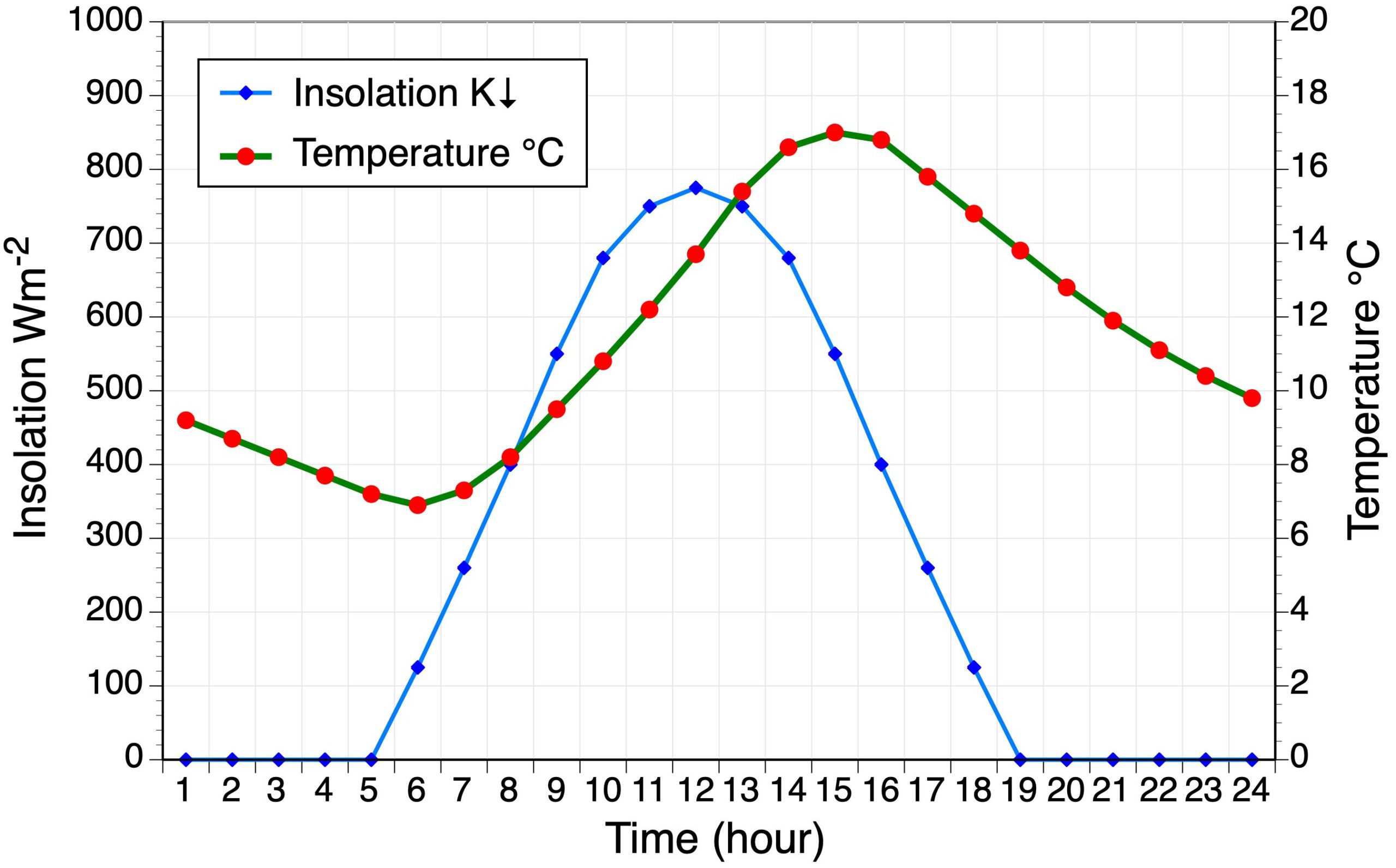
Figure 2.2. Typical relationship between insolation (K↓) and surface air temperature (T) over a 24-hour period. Location is in the mid-latitudes date is late March or mid-September and the sky in this example is free of clouds. Image Copyright: Michael Pidwirny.
The diurnal temperature range is controlled by a number of factors, of which the most important one is the moisture content of the air. Water vapour and clouds in the atmosphere reduce the daily range of temperature by absorbing the Earth’s longwave radiation at night and by reducing the amount of daytime insolation received by the ground. Counter-radiation by the atmospheric water vapour and other greenhouse gases directs absorbed longwave radiation back to the surface where it can be absorbed again to heat the ground. This process can be simply demonstrated by examining the diurnal temperature range of consecutive days where we go from clear cloudless skies to complete overcast.
Seasonal variations in the amount of solar radiation received tend to be the primary control of annual variations in temperature. In general, regions close to the Equator have small annual variations in temperature because of the small variations in the amount of insolation received over a year. Yet, as we move away from the Equator, relationships between the time of year, latitude, day length, and solar angle cause greater variations in insolation, and thus temperatures, on an annual basis.
THE SPATIAL DISTRIBUTION OF TEMPERATURE
Variations in globally distributed meteorological phenomena such as surface air temperature can be illustrated on isoline maps. Isoline is the generic term used to describe a series of non-intersecting lines that join or connect points of equal value. Isoline maps can be drawn to illustrate the distribution of a variety of meteorological variables. When these maps are constructed to display the horizontal distribution in air temperature the term isotherms is used to define lines of equal temperature. Figures 2.3 and 2.4 illustrate isothermal maps of the world for January and July, respectively. From these maps, it is obvious that differences exist in the heating characteristics of water and land surfaces. In January, isotherms are deflected southward over land and northward over water in the Northern Hemisphere. This suggests that at the same latitude in winter temperatures are higher over water and lower over land. In July, the reverse seems to hold true for the Northern Hemisphere. The isotherms are now deflected far to the north over the continents, and southward over the oceans, indicating the land has a much higher temperature than oceans at the same latitude. This phenomenon occurs because water has a much higher specific heat than the materials that make up the surface of the continents.
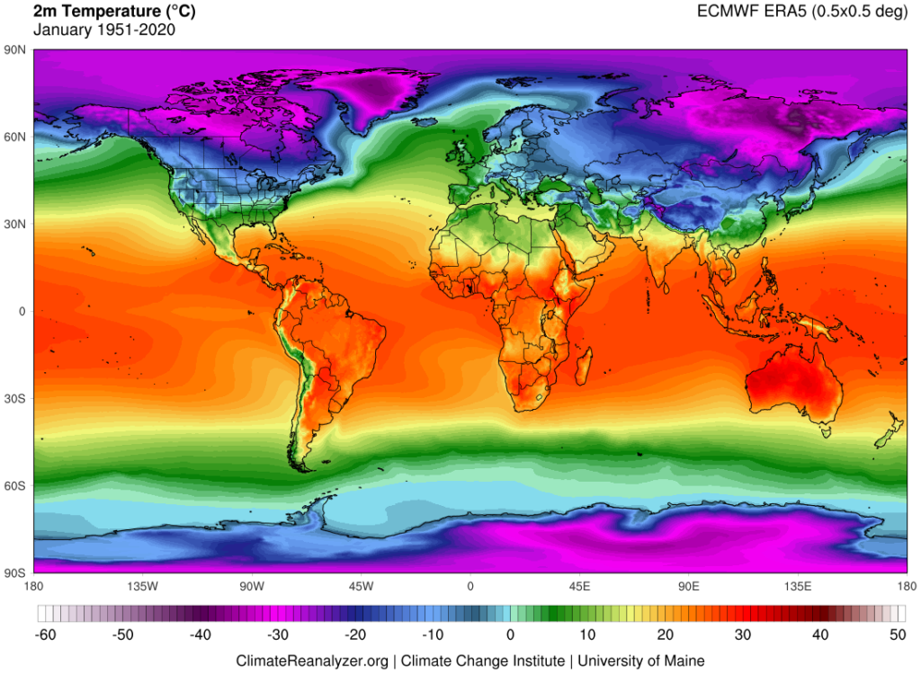
Figure 2.3. Average January air temperature at 2 meters above the Earth’s surface, 1951-2020 (data – ECMWF European Reanalysis V5). Image Source: Courtesy of Climatereanalyzer.org.
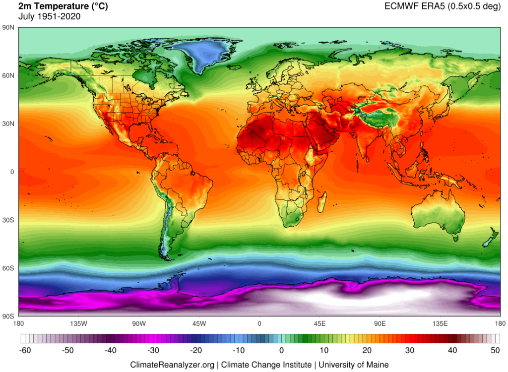
Figure 2.4. Average July air temperature at 2 meters above the Earth’s surface, 1951-2020 (data – ECMWF European Reanalysis V5). Image Source: Courtesy of Climatereanalyzer.org.
Ocean currents also exert a conspicuous effect upon global isotherms. For example, the northward-flowing Gulf Stream transports large amounts of heat from the Gulf of Mexico to northwest Europe. The Humboldt Current has the opposite effect, moving cold water from high latitudes of the Southern Hemisphere along the west coast of South America to the equator.
THE NORMAL DISTRIBUTION
Many datasets collected from various phenomena found in nature show similar patterns in terms of the variation found in observations. For datasets containing randomly selected and independent data, we often find the observations are grouped around an apparent central value. Away from the central value, the values associated with the dataset become increasingly rare with distance. When graphed, the frequency distribution of the observations in the dataset displays a pattern that resembles a bell-shaped curve (Figure 2.5). Statisticians also call this pattern a normal distribution or a normal curve. In a normal distribution, it is common for the curve’s peak to be the same value as the arithmetic average (or mean, identified by the symbol X “bar”) of all the values found in the dataset.
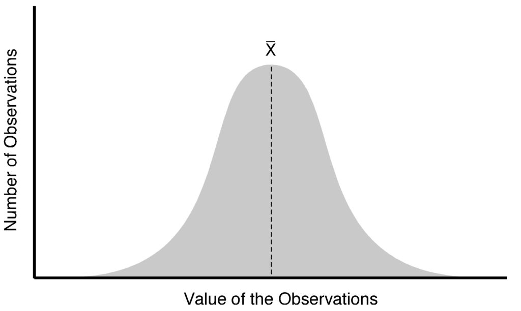
Figure 2.5. The normal distribution or bell-shaped curve. Image Copyright: Michael Pidwirny.
Another important mathematical property associated with the normal distribution is the statistic standard deviation. Standard deviation (identified by the symbol σ) is a standardized measure that can be used to describe the dispersion pattern of all the observations in a normally distributed dataset. A value of one standard deviation on either side of the mean (± 1σ) contains about 68% of the observations in a dataset (Figure 2.6). Two standard deviations above and below the mean (± 2σ) includes approximately 95% of the values in the dataset. Finally, three standard deviations either side of the mean (± 3σ) contains roughly 99% of the observations in the dataset.
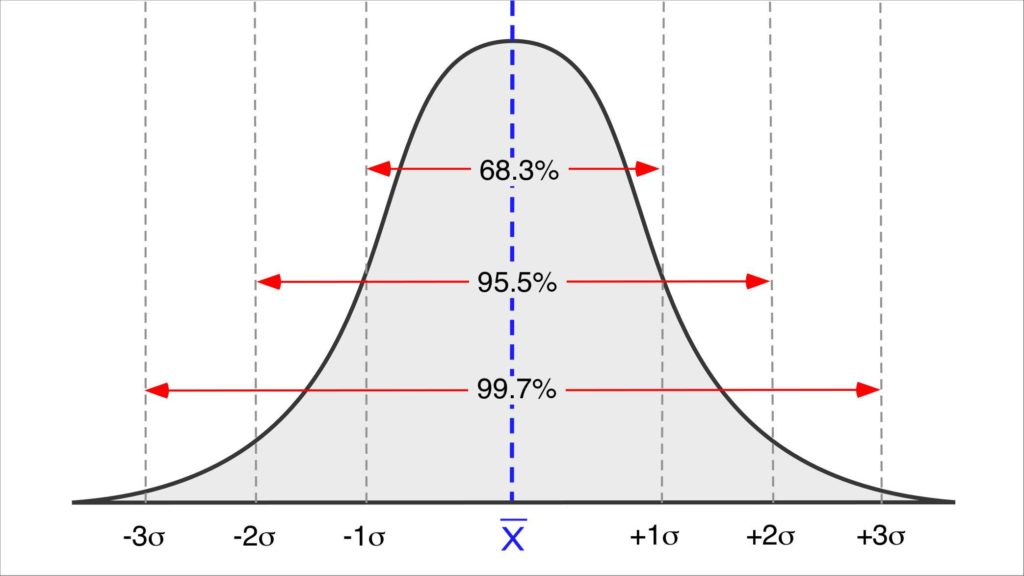
Figure 2.6. The theoretical percentage of observations from a normally distributed dataset falling ±1, ±2, and ±3 standard deviations on either side of the mean. Image Copyright: Michael Pidwirny.
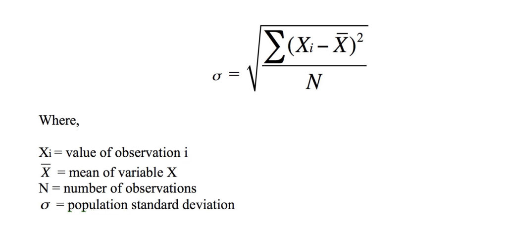
For a dataset that contains all of the observations from a population (the complete set of measurements, objects, or outcomes related to some phenomena understudy), the standard deviation is calculated:
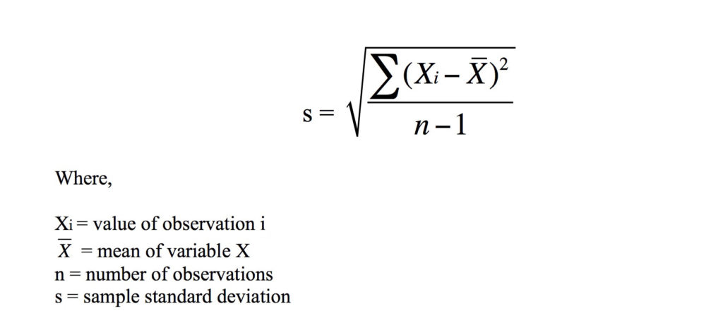
For a sample from a population, the standard deviation is calculated:
LABORATORY 2 QUESTIONS
QUESTION 1
Using the following equations, determine the values of the following in one of the three temperature scales: °Celsius, Kelvin, and °Fahrenheit.
T(°C)= 5/9 x (T(°F) – 32)
T(°C)= T(K) – 273
T(°F) = (9/5 x T(°C)) + 32
T(K)= T(°C) + 273
1.1a) Calculate the freezing point of water in °C.
_______°C
1.1b) Calculate the freezing point of water in °F.
_______°F
1.1c) Calculate the freezing point of water in K (to one decimal point).
_______K
1.2a) Calculate the boiling point of water in °C.
_______°C
1.2b) Calculate the boiling point of water in °F.
_______°F
1.2c) Calculate the boiling point of water in K (to one decimal point).
_______K
1.3a) Sun’s average surface temperature is 5778 K, covert this into °C.
_______°C
1.3b) Sun’s average surface temperature is 5778 K, covert this into °F.
_______°F
1.4a) Earth’s average surface temperature is 288 K, covert this into °C.
_______°C
1.4b) Earth’s average surface temperature is 288 K, covert this into °F.
_______°F
1.5a) The average temperature of the human body is 99°F, covert this into °C.
_______°C
1.5b) The average temperature of the human body is 99°F, covert this into K.
_______K
1.6a) The average January mean (monthly) temperature of Edmonton, Alberta, Canada is -15°C, covert this into °F.
_______°F
1.6b) The average January mean (monthly) temperature of Edmonton, Alberta, Canada is -15°C, covert this into K.
_______K
QUESTION 2
Tabulated below are vertical temperature data obtained from a radiosonde attached to a weather balloon.
| Elevation (m) | 0 | 250 | 500 | 750 | 1000 |
| Day 1 – 15:00 hrs | 20.0 | 17.0 | 14.0 | 11.5 | 9.5 |
| Day 2 – 06:00 hrs | 12.0 | 16.0 | 13.5 | 11.5 | 9.5 |
| Day 2 – 06:00 hrs | 23.0 | 18.5 | 15.0 | 12.0 | 9.5 |
On the graph (Image Copyright Michael Pidwirny) below, temperature profiles have been drawn using the data from the table above.
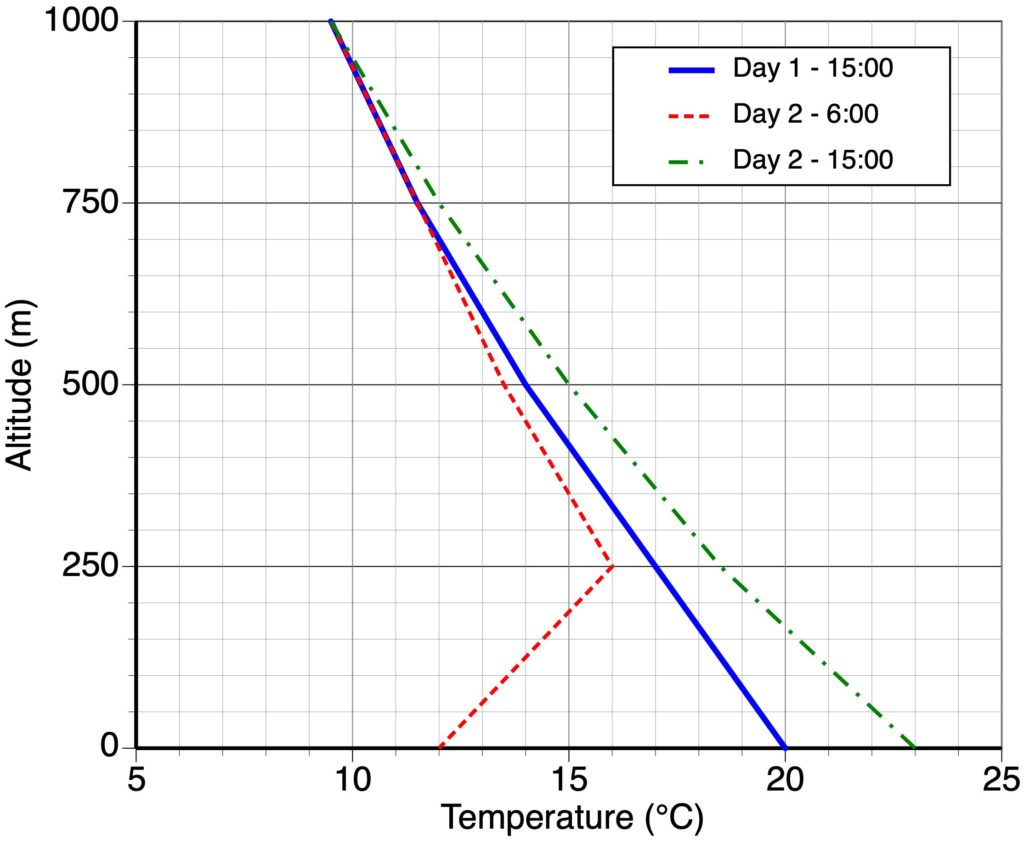
A lapse rate is simply the mathematical expression of the temperature change with elevation. Complete the following table by calculating the missing lapse rates; express your answers in mathematically correct units of °C per 1000 m, to one decimal place.
Calculate lapse rates (°C / 1000m) for the following two vertical temperature profiles.
For Day 2 – 6:00
2.1a) On Day 2 at 6:00, the calculated lapse rate per 1000 meters for the interval 0-250 meters is
_______°C/1000 m
2.1b) On Day 2 at 6:00, the calculated lapse rate per 1000 meters for the interval 250-500 meters is
_______°C/1000 m
2.1c) On Day 2 at 6:00, the calculated lapse rate per 1000 meters for the interval 500-750 meters is
_______°C/1000 m
2.1d) On Day 2 at 6:00, the calculated lapse rate per 1000 meters for the interval 750-1000 meters is
_______°C/1000 m
Day 2 – 15:00
2.2a) On Day 2 at 15:00, the calculated lapse rate per 1000 meters for the interval 0-250 meters is
_______°C/1000 m
2.2b) On Day 2 at 15:00, the calculated lapse rate per 1000 meters for the interval 250-500 meters is
_______°C/1000 m
2.2c) On Day 2 at 15:00, the calculated lapse rate per 1000 meters for the interval 500-750 meters is
_______°C/1000 m
2.2d) On Day 2 at 15:00, the calculated lapse rate per 1000 meters for the interval 750-1000 meters is
_______°C/1000 m
2.3) Why is air temperature the highest right near the Earth’s surface in both of the 15:00 hr profiles?
2.4) What processes caused the lower atmosphere to cool overnight on the Day 2 – 6:00 profile?
2.5) What processes caused the air in the lower atmosphere to warm up by 15:00 hr on Day 2?
2.6) The atmospheric condition displayed in the Day 2, 6:00 AM vertical temperature profile is called a
A Stratosphere.
B Temperature Inversion.
C Equilibrium kink.
D Temperature Diversion.
QUESTION 3
Below are the monthly mean surface air temperatures (°C) for two locations at approximately the same latitude: Vancouver, British Columbia, Canada (Latitude 49.25°, Longitude -123.10°) and Winnipeg, Manitoba, Canada (Latitude 49.89°, Longitude -97.15°) averaged for the period 1981-2010. (Note: a climate “normal” monthly average is the average of daily surface air temperature maximums and minimums throughout the month, usually over a period of 30 years.)
| Month | Vancouver | Winnipeg |
| January | 4.1 | -16.4 |
| February | 4.9 | -13.2 |
| March | 6.9 | -5.8 |
| April | 9.4 | 4.4 |
| May | 12.8 | 11.6 |
| June | 15.7 | 17.0 |
| July | 18.0 | 19.7 |
| August | 18.0 | 18.8 |
| September | 14.9 | 12.7 |
| October | 10.3 | 5.0 |
| November | 6.3 | -4.9 |
| December | 3.6 | -13.2 |
On the graph (Image Copyright Michael Pidwirny) below, are plots of monthly mean surface air temperature data for the two locations, and the data points are connected with lines.
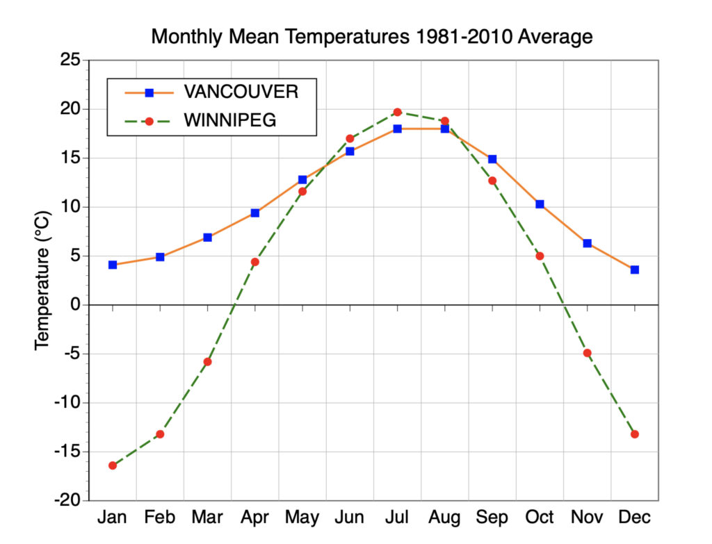
From the data in the table, calculate the following values:
3.1) Average annual surface air temperature (°C) for Vancouver.
_______°C
3.2) Average annual surface air temperature (°C) for Winnipeg.
_______°C
3.3) The annual surface air temperature range (°C) for Vancouver. (Note: “annual temperature range” is the difference between maximum monthly temperature and minimum monthly temperature.)
_______°C
3.4) The annual surface air temperature range (°C) for Winnipeg. (Note: “annual temperature range” is the difference between maximum monthly temperature and minimum monthly temperature.)
_______°C
3.5) Explain the difference in magnitude of the annual ranges of temperature for these two locations. Keep in mind that these two locations are at similar latitudes. Which city has a more “continental” climate?
QUESTION 4
The graphs (Image Copyright Michael Pidwirny) below describe hourly fluctuations in surface air temperature and potential insolation for Kelowna, British Columbia, Canada (Latitude 49.89°, Longitude -119.50°). Data is shown for two specific days: February 14, 2005 and August 12, 2005. Explain the patterns in air temperature using the insolation data.
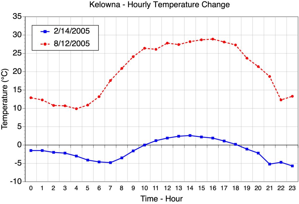
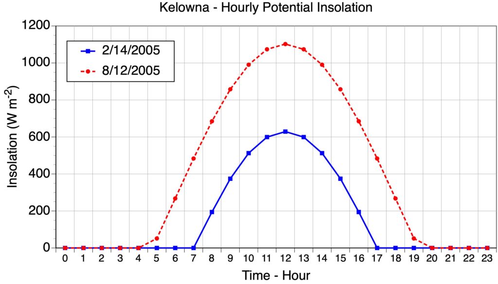
4.1a) At what time (hour) did minimum surface air temperature occur on February 14, 2005?
_______
4.1b) At what time (hour) did minimum surface air temperature occur on August 12, 2005?
_______
4.1c) Explain why the morning minimum surface air temperature on the two days occurs at different times.
4.2a) At what time (hour) did maximum surface air temperature occur on February 14, 2005?
_______
4.2b) At what time (hour) did maximum surface air temperature occur on August 12, 2005?
_______
4.2c) Explain the difference in the timing of maximum daily surface air temperature for both days.
4.3) Why are the daily surface air temperatures on February 14, 2005 much cooler than those that occurred on August 12, 2005?
QUESTION 5
Use the following web link to go to Climate Reanalyzer, Monthly Reanalysis Maps.
https://climatereanalyzer.org/reanalysis/monthly_maps/
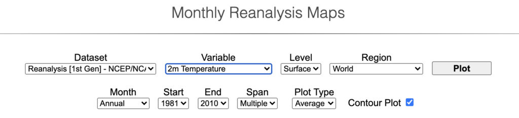
Create a global map showing annual average 2 meter temperature °C for the 30-year period 1981-2010 with the following inputs.
Answer the following questions.
5.1) In general, the warmest surface temperatures are found at
A the equator.
B 25° South Latitude.
C 25° North Latitude.
D 50° South Latitude.
E 50° North Latitude.
5.2) In general, the coldest surface temperatures are found at
A Antarctica.
B the Arctic.
C the center of Greenland.
D Siberia.
5.3) At 50° North, the warmest surface temperatures are found on
A land surfaces.
B ocean surfaces.
C the center of Greenland.
D Siberia.
5.4) Explain your answer for question 5.3.
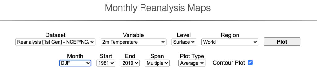
Create a SECOND global map showing Winter Season (DJF – December/January/February) average 2 meter temperature °C for the 30-year period 1981-2010 with the following inputs. Create this map in a separate window so you can make comparisons to the annual average.
Answer the following questions.
5.5) In general, the warmest surface temperatures are found
A at the equator.
B over Australia.
C over Mexico.
D over Northern Africa.
E over Canada.
5.6) In general, the coldest surface temperatures are found at
A Antarctica.
B the Arctic.
C the Southern Ocean around Antarctica.
D Atlantic Ocean in between Canada and Europe.
Create a THIRD global map showing Summer Season (JJA – June/July/August) average 2 meter temperature °C for the 30-year period 1981-2010 with the following inputs. Create this map in a separate window so you can make comparisons to the annual average.

Answer the following questions.
5.7) In general, the warmest surface temperatures are found
A at the equator.
B over Australia.
C over Mexico.
D over Northern Africa.
E over Canada.
5.8) In general, the coldest surface temperatures are found at
A Antarctica.
B the Arctic.
C the Southern Ocean around Antarctica.
D Atlantic Ocean in between Canada and Europe.
5.9) Explain why surface temperatures over Australia have cooled off when compared to Winter (DJF), 1981-2010?
QUESTION 6
The Microsoft Excel file Lab_2_Kamloops_Temp_Data.xlsx shows the monthly and annual mean surface air temperatures for Kamloops, British Columbia, Canada for the period 1901-2019. At the end of each data column means, standard deviations (σ), Mean + 2σ, and Mean – 2σ have been calculated for the entire time series. The mean has been calculated by adding together all the values in the data set and dividing by the number of values in the data set.
The following graph (Image Copyright Michael Pidwirny), plots the average monthly surface air temperature for Kamloops, connecting the data points with straight lines. Also, for each month plot “error bars” representing two standard deviations (± 2σ) of dispersion around the mean value have been drawn.
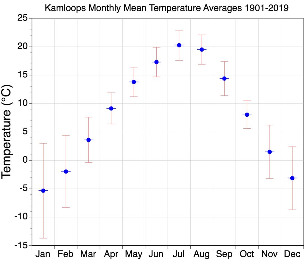
For January and July, list the years in which the average surface air temperatures were higher or lower than 2 standard deviations (± 2σ) than the averages in these months. January has been done for you as an example.
January Mean = -5.3, ± 2σ = 3.0 to -13.7
Higher than +2s: No years have values greater than +2s.
Lower than -2s: 1950, 1916, 1930, 1969, 1907, 1937, and 1957.
Answer the following questions for July.
July Mean = 20.3, ± 2σ = 22.9 to 17.6
6.1) For July, are there any years with a monthly mean temperature that is higher than +2σ? Please list them.
6.2) For July, are there any years with a monthly mean temperature that is lower than -2σ? Please list them.
6.3) For July, would you consider the years listed in questions 6.1 and 6.2 to be anomalies in the climate record of Kamloops? Explain relative to the normal distribution concept.
6.4) Generally, in which season does Kamloops have the GREATEST interannual variations in surface air temperature at shown by the calculation of standard deviation?
A Winter (December, January, and February)
B Spring (March, April, and May)
C Summer (June, July, and August)
D Fall (September, October, and November)
6.5) Generally, in which season does Kamloops have the LEAST interannual variations in surface air temperature at shown by the calculation of standard deviation?
A Winter (December, January, and February)
B Spring (March, April, and May)
C Summer (June, July, and August)
D Fall (September, October, and November)
IMAGE CREDITS
Figure 2.1: Image Copyright Michael Pidwirny.
Figure 2.2: Image Copyright Michael Pidwirny.
Figure 2.3: Image Courtesy of Climatereanalyzer.org.
Figure 2.4: Image Courtesy of Climatereanalyzer.org.
Figure 2.5: Image Copyright Michael Pidwirny.
Figure 2.6: Image Copyright Michael Pidwirny.
QUESTION ANSWER SHEET
FIGURES AND TABLES – PDF FILES
MICROSOFT EXCEL DATA FILES
Lab 2_Winnipeg_and_Vancouver_Monthly Temp.xlsx
Lab_2_Lethbridge_Temp_Data.xlsx
Lab_2_Penticton_Temp_Data.xlsx
This Laboratory Exercise is Licensed Under Attribution-NonCommercial-NoDerivatives 4.0 International (CC BY-NC-ND 4.0).
Updated April 5, 2021
Temperature is defined as the measure of the average speed of atoms and molecules. The higher the temperature the faster they move.
Heat is defined as energy in the process of being transferred from one object to another because of the temperature difference between them. In the atmosphere, heat is commonly transferred by conduction, convection, advection, and radiation.
Is defined as the capacity for doing work. Energy can exist the following forms: radiation; kinetic energy; potential energy; chemical energy; atomic energy; electromagnetic radiation; electrical energy; and heat energy.
A temperature of -273.15°C or -459.67°F or 0 Kelvin. At this temperature atomic motion essentially stops and the kinetic energy of atoms is at a minimum.
Scale used in the measurement of temperature. In this scale, water boils at 212° and freezes at 32°. It is used in only a few countries, most notably the United States where it is used for weather forecasting and other non-scientific purposes.
Common scale used in the measurement of temperature. In this scale, water boils at 100° and freezes at 0°. This scale is used in most countries. One notable exception is the United States where the Fahrenheit scale is used for weather forecasting and other non-scientific purposes.
Common scale used in science and engineering for measuring temperature. In this scale, absolute zero is 0 Kelvins, water boils at 373.15 Kelvins, and freezes at 273.15 Kelvins. One of the seven base measurement units used in the International System of Units (SI).
Device used to measure temperature. A variety of different devices have been invent to measure temperature by converting some physical change into a numerical value. Some of the methods employed in these devices include thermal expansion of substances, pressure changes associated with substances, and the measurement of electromagnetic radiation emission.
In terms of meteorology and weather forecasting, this term refers to the temperature of the air about 1.5 meters (4.5 feet) above the ground surface where it is routinely measured at weather stations on land surfaces.
A meteorological thermometer designed to record the maximum temperature over a set time interval, usually 24 hours (midnight to midnight). Liquid-in-glass type of maximum thermometers have a bore that is narrowed between the reserve bulb and graduated portion of the glass stem. With a rise in temperature, the mercury found in reserve bulb pushes past the constriction and up into the graduated section as long as temperature continues to increase. The mercury in the graduated section does not fall back into the reserve bulb because of the constriction, and as a result, the highest temperature reached is recorded.
A meteorological thermometer designed to record the minimum temperature over a set time interval, usually 24 hours (midnight to midnight). Liquid-in-glass type of minimum thermometers are normally filled with red-colored alcohol and have a black metal slider that can move up and down through the bore. When temperature drops, the black metal slider is pushed by the retreating top surface of the alcohol because of surface tension down the bore. When temperature begins to rise again, the slider is designed not to move thereby permanently recording the minimum temperature. The slider is reset by positioning the thermometer upside down.
A specially designed housing for meteorological instruments used to keep measurements standardize around the world (Image Source: Wikipedia Commons). This housing consists of wooden box painted white with double louvered sides. It is mounted on a stand 1.5 meters or 4.5 feet (this does vary from country to country between 1.2 to 1.8 meters or 3.9 to 5.9 feet) above the ground surface and contains maximum thermometer, minimum thermometer, barometer, dry-bulb thermometer, and wet-bulb thermometer.
The rate at which air temperature decreases with an increase in altitude. Represents the vertical temperature gradient in the atmosphere. Meteorologists routinely measure the atmospheric lapse rate at weather stations via radiosondes.
An international reference unit of pressure. 1 atm = 101325 pascals (Pa) = 101.325 kilopascals (kPa) = 1013.25 millibars (mb).
The tropopause is a relatively thin atmospheric transition layer found between the troposphere and the stratosphere. The height of this layer varies from 8 to 16 kilometers (5.0 to 10.0 miles) above the Earth's surface.
The rate of air temperature increase or decrease with altitude. The average ELR in the troposphere is an air temperature decrease of 6.5°C per 1,000 meters (3.6°F per 1,000 feet) rise in elevation. Also called normal lapse rate.
Situation where a layer of warmer air exists above the Earth's surface in a normal atmosphere where air temperature decreases with altitude. In the warmer layer of air, temperature increases with altitude.
Layer in the atmosphere found from the surface to a height of between 8 to 16 kilometers (5.0 to 10.0 miles) of altitude [average height 11 kilometers (6.8 miles)]. The troposphere is thinnest at poles and gradually increases in thickness as one approaches the equator. This atmospheric layer contains about 80% of the total mass of the atmosphere. It is also the layer where the majority of our planet's weather occurs. Maximum air temperature occurs near the Earth's surface in this layer. With increasing altitude air temperature drops uniformly with increasing height at an average rate of 6.5°C per 1,000 meters (3.6°F per 1,000 feet) (commonly called the Environmental Lapse Rate), until an average temperature of -56.5°C (-70°F) is reached at the top of the troposphere.
Atmospheric layer found at an average altitude of 11 to 50 kilometers (6.8 to 31.1 miles) above the Earth's surface. Within the stratosphere exists the ozone layer. Ozone's absorption of ultraviolet sunlight causes air temperature within the stratosphere to increase with altitude.
The stratopause is a relatively thin atmospheric transition layer found between the stratosphere and the mesosphere. The height of this layer is about 50 kilometers (31 miles) above the Earth's surface.
Atmospheric layer found between the stratosphere and the thermosphere. The mesosphere is located at an average altitude of 50 to 80 kilometers (31 to 50 miles) above the Earth's surface. Air temperature within the mesosphere decreases with increasing altitude.
Thin boundary layer found between the mesosphere and the thermosphere. The mesopause is found at an average altitude of 80 kilometers (50 miles). The coldest temperatures in the atmosphere are found in the mesopause.
Atmospheric layer above the mesosphere (above 80 kilometers or 50 miles) characterized by air temperatures rising rapidly with height. The thermosphere is the hottest layer in the atmosphere. In the thermosphere, gamma, X-ray, and specific wavelengths of ultraviolet radiation are absorbed by certain gases in the atmosphere. The absorbed radiation is then converted into heat energy. Temperatures in this layer can be greater than 1,200°C (2,190°F).
A form of electromagnetic radiation with a wavelength roughly between 0.7 and 100 micrometers (µm). Also called infrared radiation.
Direct or diffused shortwave solar radiation that is received in the Earth's atmosphere or at its surface.
Heat energy that can be measured by a thermometer and thus potentially sensed by humans.
Process that involves the transfer of mass and heat energy using vertical motions through a fluid substance like air or water.
The balance between incoming and outgoing shortwave and longwave radiations. Mathematically expressed as:
Q* = (K + k)(1 - a) - L⬆ + L⬇
where Q* is surface net radiation (global annual values of Q* = 0, because input equals output, local values can be positive or negative), K is surface direct shortwave (solar) radiation, k is diffused shortwave (solar) radiation (scattered insolation) at the surface, a is the albedo of surface, L⬇ is atmospheric counter-radiation (greenhouse effect) directed to the Earth's surface, and L⬆ is longwave radiation lost from the Earth's surface.
The daily range between maximum and minimum values of some meteorological like surface air temperature, relative humidity or atmospheric pressure.
Lines joining points of equal value for some measurable characteristic shown on a map.
Lines (isolines) on a map joining points of equal temperature.
Is the heat capacity of a unit mass of a substance or heat needed to raise the temperature of 1 gram (g) of a substance 1 degree Celsius.
A common probability distribution displayed by a representative data sample or the whole population of some quantitatively measurable variable. If the values of this distribution are plotted on a graph's horizontal axis and their frequency on the vertical axis, the pattern displayed is symmetric and bell-shaped (see graph). The central value in this type of frequency distribution is usually mean (arithmetic average of all the values measured for the variable), and this value represents the central peak of the distribution and the most frequently occurring value. Also called normal curve and bell-shaped curve.
Statistical measure of central tendency in a set of data. The mean is calculated by adding all of the data values and dividing this quantity by the total number of data values. Also called the average.
A statistical measure of the dispersion of observation values in a data set around the mean (average). Calculated by determining the square root of the variance.
A statistical population is the entire collection of people, animals, plants or things from which we may collect data from and analyze this data using qualitative or quantitative techniques.
