Michael Pidwirny
LABORATORY 4: MID-LATITUDE CYCLONES, WEATHER MAPS, AND FORECASTING
LEARNING GOALS
In this laboratory, we will examine the process of mid-latitude cyclone development and will learn some basic techniques of weather forecasting in the middle latitudes.
Upon completion of this laboratory you will be able to:
- Understand the role of air masses, fronts, and mid-latitude cyclones in producing weather on our planet.
- Interpret present climatic conditions from synoptic weather maps.
- Use computer model forecasts to predict weather in the immediate future.
AIR MASSES AND FRONTS
An air mass is a large body of air of relatively similar temperature and humidity characteristics covering thousands of square kilometers. Typically, air masses are classified according to the characteristics of their source region or area of formation. A source region can have one of four temperature attributes: Equatorial, tropical, polar, and arctic (this terminology is at first somewhat confusing because “polar” does not in fact refer to air masses originating at the poles). Air masses are also classified as being either continental or maritime in terms of moisture characteristics. Combining these two categories, several possibilities are commonly found associated with weather in North America (Figure 4.1): maritime polar (mP), continental polar (cP), maritime tropical (mT), continental tropical (cT), and continental arctic (cA).
Frequently two air masses, especially tropical and polar, develop a sharp boundary or interface. Such an area of intensification is called a frontal zone, or more commonly, a front. At a front, warmer air will override the denser, colder air. This means that where air masses converge, the warmer air is uplifted. This uplifting causes condensation and cloud formation to occur and the possibility of precipitation along the frontal boundary. Notice in Figure 4.1 where air masses with different characteristics usually meet, and where frontal lifting might occur.
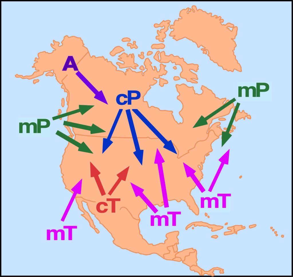
Figure 4.1. Generalized map of air mass source regions and trajectories for North America. Note: not all of these air masses are present at any given time. Image Copyright: Michael Pidwirny.
Different types of front occur; see Table 4.1 for weather conditions associated with the common ones.
Table 4.1. Generalized weather conditions associated with surface fronts.
| AS A COLD FRONT PASSES: | |
| Temperature: | decreases |
| Moisture: | absolute humidity and dewpoint decreases as front passes |
| Wind Direction: | SW winds change to NW winds |
| Air pressure: | may decrease during frontal passage, then rise afterwards |
| Clouds and Precipitation: | cumuliform clouds common; heavy showers; possible thunderstorms; then rapid clearing |
| AS A WARM FRONT PASSES: | |
| Temperature: | increases |
| Moisture: | absolute humidity and dewpoint increases as front passes |
| Wind Direction: | SE winds change to SW winds |
| Air pressure: | may decrease during frontal passage, then stabilize |
| Clouds and Precipitation: | gradual increase and lowering of stratiform cloud cover followed by extended period of steady, widespread precipitation; partial or full clearing after frontal passage |
| OCCLUDED FRONT: | |
| Temperature: | cold before and after passage, but temperature may go up or down depending on the type of occlusion |
| Moisture: | high relative humidity and low or moderate dew point before and after passage |
| Wind Direction: | southerly before passage; more westerly after passage |
| Air pressure: | may decrease during frontal passage, then rise afterwards |
| Clouds and Precipitation: | increase and lowering of cloud cover followed by extended period of precipitation (freezing rain or snow is possible), followed by clearing |
| STATIONARY FRONT: | |
| Weather: | extended cloudiness; possible light precipitation; temperature, moisture, wind, and air pressure remain relatively steady |
MID-LATITUDE CYCLONES
Mid-latitude cyclones or extratropical cyclones are large traveling vortices (rotating air) about 2000 km in diameter with centers of low pressure. An intense mid-latitude cyclone may have a surface pressure of less than 970 mb, compared to the average sea level pressure of 1013 mb. Surface winds around the low blow cyclonically inwards (as you learned in Lab 3). Precipitation is typically located at the center of the low and along the fronts. Mid-latitude cyclones generally travel eastward, although movement is often controlled by jet stream winds in the upper troposphere. The mid-latitude cyclone is rarely motionless and commonly travels about 1200 km in one day. Its direction of movement is generally eastward. The precise movement of this weather system is controlled by the orientation of the polar jet stream in the upper troposphere. An estimate of future movement speed of the mid-latitude cyclone can be determined by the winds directly behind the cold front. If the winds are 70 km per hour, the cyclone can be projected to continue its movement along the ground surface at this velocity. Normally, individual frontal cyclones exist for about 3 to 10 days moving in a generally west to east direction. Frontal cyclones are the dominant weather event of the Earth’s mid-latitudes forming along the polar front (Figure 4.2).
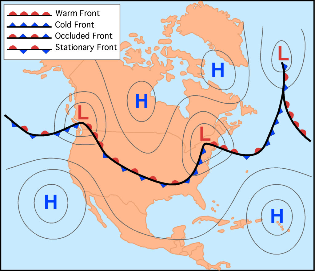
Figure 4.2. A series of mid-latitude cyclones forming along the polar front (line with half circle and triangle symbols). In the illustration, the low pressure center of the mid-latitude cyclones is identified by a letter L. The systems located along the west and east coast of North America are in the middle stage of their life. The mid-latitude cyclone east of Greenland is at the end of its life cycle. In their mature stage, mid-latitude cyclones have a warm front on the east side of the storm’s center and a cold front to the west. The cold front travels faster than the warm front. Near the end of the storm’s life, the cold front catches up to the warm front causing a condition known as occlusion, or an occluded front. Image Copyright: Michael Pidwirny.
Figure 4.3 describes the patterns of wind flow, surface pressure, fronts, and zones of precipitation associated with a mid-latitude cyclone in the Northern Hemisphere. Around the low, winds blow counter-clockwise and inwards (clockwise and inward in the Southern Hemisphere). West of the low, cold air traveling from the north and northwest creates a cold front extending from the cyclone’s center to the southwest. Southeast of the low, northward moving warm air from the subtropics produces a warm front. Precipitation is located at the center of the low and along the fronts where air is being uplifted.
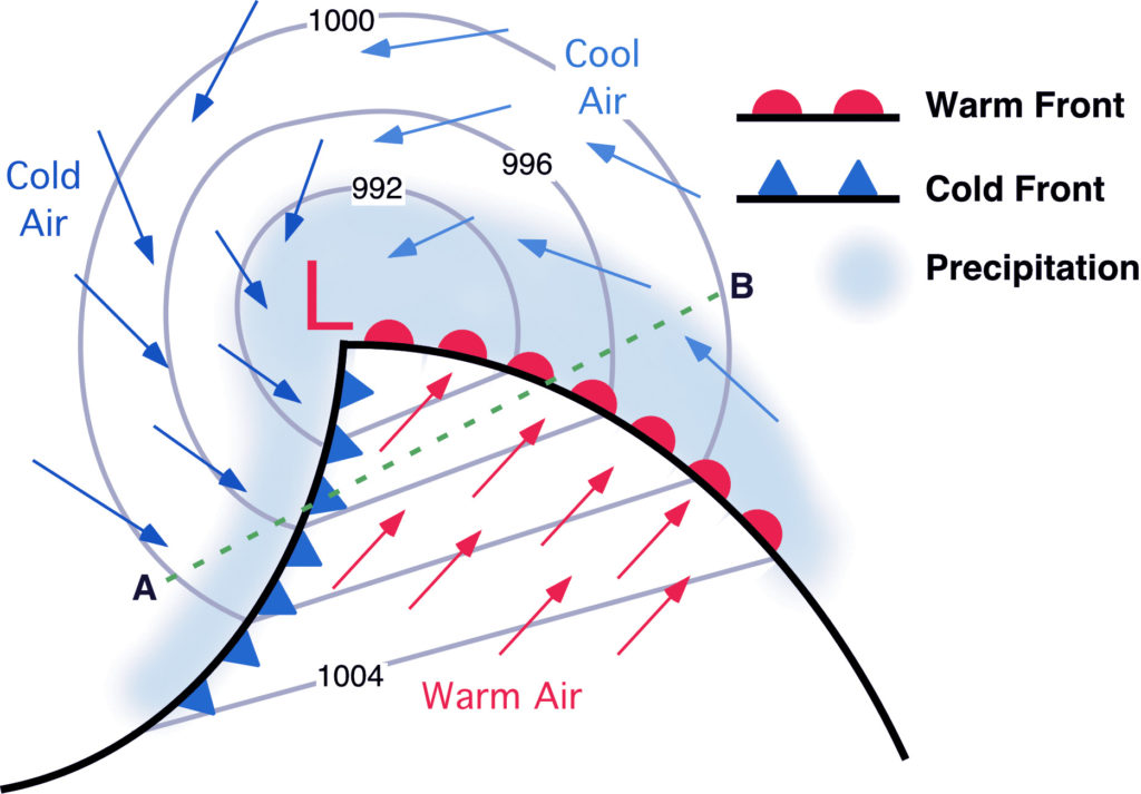
Figure 4.3. Fronts, winds patterns, pressure patterns, and precipitation distribution found in an idealized mature mid-latitude cyclone. See Figure 4.4 for atmospheric cross-section A-B above. Image Copyright: Michael Pidwirny.
Figure 4.4 describes a vertical cross-section through a mature mid-latitude cyclone. In this cross-section, we can see how air temperature changes as we move from a position ahead of the warm front (right side of diagram) to one behind the cold front (left side). Behind the cold front, forward-moving colder, denser air causes the uplift of the warmer, lighter air in advance of the front. Because this uplift is relatively rapid along a steep frontal gradient, the condensed water vapor quickly organizes itself into cumulus and then cumulonimbus clouds. Cumulonimbus clouds produce heavy precipitation and can develop into severe thunderstorms if conditions are right. Along the gently sloping warm front, the lifting of moist air produces first nimbostratus clouds followed by altostratus and cirrostratus. Precipitation is less intense along this front, varying from moderate to light showers some distance ahead of the surface location of the warm front.
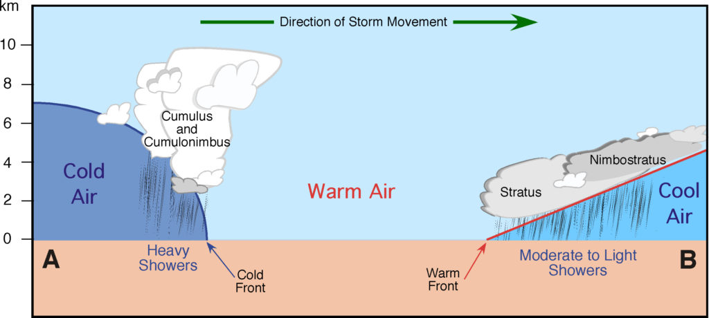
Figure 4.4. Vertical cross-section of the line A-B in Figure 4.3. Image Copyright: Michael Pidwirny.
Figure 4.5 shows a simplified model of cyclogenesis. The cyclone begins as a weak disturbance along a stationary front where colder air from Polar regions meets warmer air from subtropical regions (Figure 4.5 – stage 1). The collision of these two air masses results in the uplift of the warm air into the upper atmosphere creating a cyclonic spin around a low-pressure center (Figure 4.5 – stages 2-3). Associated with this center are the cold and warm fronts. Notice that colder air pushing into warmer air produces a cold front, while warmer air pushing into colder air results in a warm front. The warmer air south of the low’s center and between the two fronts is known as the warm sector. Cold fronts usually move along the Earth’s surface at velocities greater than the warm front. As a result, the late stages of cyclogenesis occur when the cold front overtakes the warm front causing the air in the warm sector to be lifted into the upper atmosphere (Figure 4.5 – stage 4). The resulting boundary between the cold and cool air masses is called an occluded front. This usually dissipates within a couple of days, winds subside, and the frontal zone becomes stationary again (Figure 4.5 – stages 5-6).
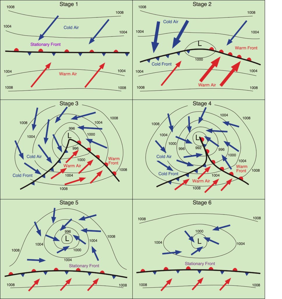
Figure 4.5. Simplified stages in the life cycle of a mid-latitude cyclone (Northern Hemisphere). See text for explanation. Image Copyright: Michael Pidwirny.
THE WEATHER MAP
The surface or synoptic weather map is one of the most important tools used for forecasting weather and contains various types of meteorological information gathered from hundreds of weather stations. In Canada and the USA, about 29,000 stations observe the weather on a daily basis. Of these stations, about 1300 are primary weather stations making complete synoptic observations at 00, 06, 12 and 18 hours Universal Time (UTC or Z; this is equivalent to Greenwich Mean Time, GMT).
Figure 4.6 shows a simple synoptic weather map for April 17, 2020 produced by the NOAA’s (National Oceanic and Atmospheric Administration) Weather Prediction Center in the United States and accessed from their Daily Weather Map website. On this map, we can see a mature mid-latitude cyclone with its low pressure center located in the state of Missouri. Extending from the east of the low is a warm from, while a cold front extends to the south-southeast. We will examine this particular weather system in greater detail later on in this lab.
Figure 4.6. Modern style surface weather map for April 17, 2020 at 7:00 EST or 11:00 UTC. Map Source: National Oceanic and Atmospheric Administration, Weather Prediction Center, Daily Weather Map website.
Government organizations like NOAA and Environment and Climate Change Canada (Weather Information), have also produced more complex weather maps as shown in Figure 4.7. Weather conditions at the station level on these old-style weather maps are represented by a complex system of symbols and numbers as shown in Figure 4.8. Typical weather station observations include: surface air temperature, dew point temperature, wind speed, wind direction, the amount and type of cloud cover, precipitation, and atmospheric pressure (current, and the change over the previous three hours). Information from the world’s synoptic stations is transmitted electronically to a processing center where computer maps and forecasts are constructed (e.g., Figure 4.6).

Figure 4.7. North American 1990s surface weather analysis map for Saturday, April 13, 1996 at 12 UTC. Map Source: National Oceanic and Atmospheric Administration, Weather Prediction Center, Historical Archive of North American Analyses Webpage.
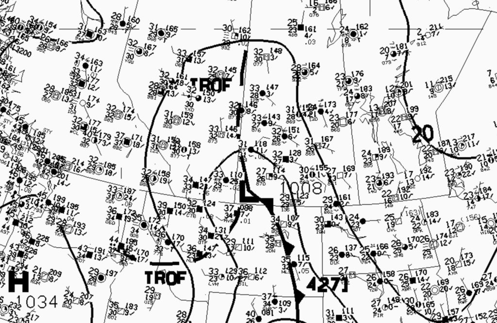
Figure 4.8. Zoomed in section of the synoptic weather map found in Figure 4.7. At this scale, you can see the coded weather information around each weather station. Map Source: National Oceanic and Atmospheric Administration, Weather Prediction Center, Historical Archive of North American Analyses Webpage.
DECODING A WEATHER STATION MODEL
Actual weather conditions at the station level are shown on synoptic weather maps by a number of symbols and shorthand code. The figure below shows a typical weather station with some of the more important weather measurements typically displayed (top-left). The other information shown on this graphic explains the symbol and shorthand coding systems used to display recorded weather measurements. Note that the temperature-related measurements are for a synoptic weather map created outside the USA, which uses Fahrenheit instead of Celsius.
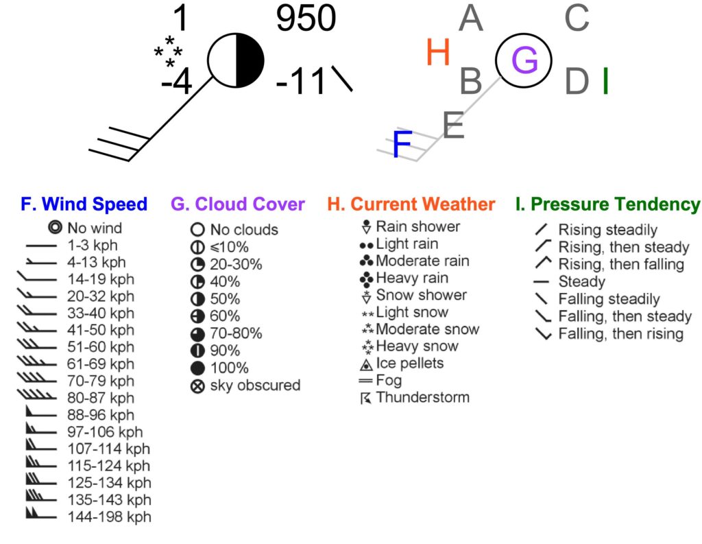
The following list helps interpret the weather station model shown. Use the graphic in the top-right corner to decipher the symbols and shorthand code.
A = Current air temperature at the weather station, which is 1°Celsius. In the USA, temperature is measured in Fahrenheit.
B = Current dew point temperature at the weather station, which is -4°Celsius (Fahrenheit for USA maps). In the USA, dew point temperature is measured in Fahrenheit.
C = Current atmospheric pressure adjusted for sea level at the weather station, which in our example is 995.0 millibars (mb). Pressure at sea level usually varies between 970.0 and 1050.0 mb. Meteorologists represent this measurement in shorthand form on a synoptic weather map. The shorthand form involves dropping the initial 9 or 10 from the number and removing the decimal. For example, if air pressure at a weather station was measured as 1013.2mb, this would be shown as 132 on the weather map.
D = Atmospheric pressure change at the weather station in the last 3 hours, which is a decrease (-) of 1.1 mb. Note on the synoptic weather map the decimal point is removed from the reading.
E = Wind direction the direction of wind blowing into the weather station (where is the wind coming from), which is southwest. The following graphic shows the major cardinal directions.
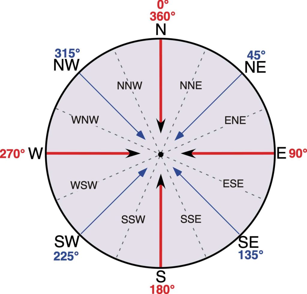
Figure 4.9. Wind compass describing the sixteen principal bearings used to measure wind direction. This system is based on the 360 degrees found in a circle. Image Copyright: Michael Pidwirny.
F = Wind speed at the weather station, which is 51-60 kilometers per hour (kph). Note in the USA wind speed is measured in knots and 10 knots = 18.5 kph = 11.5 mph.
G = Sky covered by clouds at the weather station, which is 50% covered by clouds.
H = Current weather conditions at the station, which is heavy snow.
I = Atmospheric pressure tendency over the last 3 hours at the weather station, which is falling steady.
The following YouTube video provides more instruction on interpreting weather station models:
LABORATORY 4 QUESTIONS
QUESTION 1
Using the information on “decoding a weather station model” found above, decipher the weather information from the following Canadian weather station:

1.1) What is the current air temperature in °C?
1.2) What is the current dew point temperature in °C?
1.3) Wind direction is from the
A Northeast.
B Southwest.
C North.
D South.
1.4) Wind velocity at the location is
A 14-19 kilometers per hour.
B 20-32 kilometers per hour.
C 33-40 kilometers per hour.
D 41-50 kilometers per hour.
1.5) Clouds cover how much of the sky?
A 20-30%.
B 40%.
C 50%.
D 60%.
1.6) Atmospheric pressure in millibars at the location is
______ mb.
1.7) The change in atmospheric pressure in millibars over the last 3 hours at the location is
______ mb.
1.8) The pressure tendency at the weather station is
A rising steadily.
B rising, then steady.
C rising, then falling.
D steady.
1.9) Describe the precipitation occurring at the weather station?
A Light rain.
B Rainshower.
C Light snow.
D Moderate rain.
QUESTION 2
Please review the following YouTube video on “How to read a synoptic chart“.
The following three synoptic weather maps (charts) found in Questions 2, 3, and 4 (Figures 4.10, 4.11, and 4.12) were generated by NOAA’s Weather Prediction Center in the United States. Each of these maps displays the actual weather experienced daily at 7:00 EST or 11:00 UTC (Z) on April 16, 17, and 18, 2020. These maps are also available in a single PDF file called Lab4_Questions_234_Maps.pdf located at the end of this lab. This PDF document is useful for answering the questions that follow. Please note that this PDF file allows you to zoom in on each of the maps to get a closer look at individual weather station information.
The following two YouTube videos were constructed using 47 hourly synoptic map forecasts between April 16, 2020 at 7:00 EST or 11:00 UTC (Z) to April 18, 2020 at 7:00 EST or 11:00 UTC (Z). These maps were collected from Climate Reanalyzer’s Hourly Forecast Maps webpage. The first video shows the hourly change in precipitation rate (mm per hour) and mean sea level pressure (mb).
Video – Precipitation (mm per hour) and Air Pressure (mb) Variations, April 16 to 18, 2020
The second video shows the hourly change in air temperature at 2 meters above the ground surface (°F).
Video – Temperature (°F) Variations, April 16 to 18, 2020
Review the two videos above noting the spatial changes in precipitation rate, mean sea level pressure, and air temperature over the 47 hours animated before attempting Questions 2, 3, and 4.
On the April 16, 2020 surface weather map, an area of low pressure (red L) is located in southern Utah. The mid-latitude cyclone shown here is at the early stages of cyclogenesis. The questions that follow are related to this storm system.
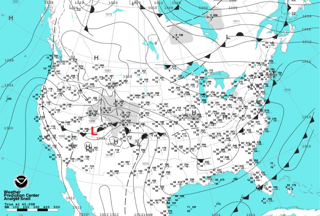
Figure 4.10. Surface weather map and station weather for Thursday April 16, 2020 at 7:00 EST or 11:00 UTC (Z). Map Source:National Oceanic and Atmospheric Administration, Weather Prediction Center, Daily Weather Map website.
2.1) What is the approximate atmospheric pressure of the storm’s low center? Note that this value is usually found on the synoptic map in a font smaller than the one used to identify isobars – look above the L.
2.2) What type of front is found west of storm’s low pressure center?
A Stationary front.
B Occluded front.
C Warm front.
D Cold front.
2.3) What type of front is found east of storm’s low pressure center?
A Stationary front.
B Occluded front.
C Warm front.
D Cold front.
2.4) Wind flow around the low pressure center is
A clockwise.
B counter-clockwise.
QUESTION 3
On the April 17, 2020 surface weather map, the low pressure center of a mid-latitude cyclone (red L) has moved and is now influencing the eastern United States (Figure 4.11). The questions that follow are related to this storm system.
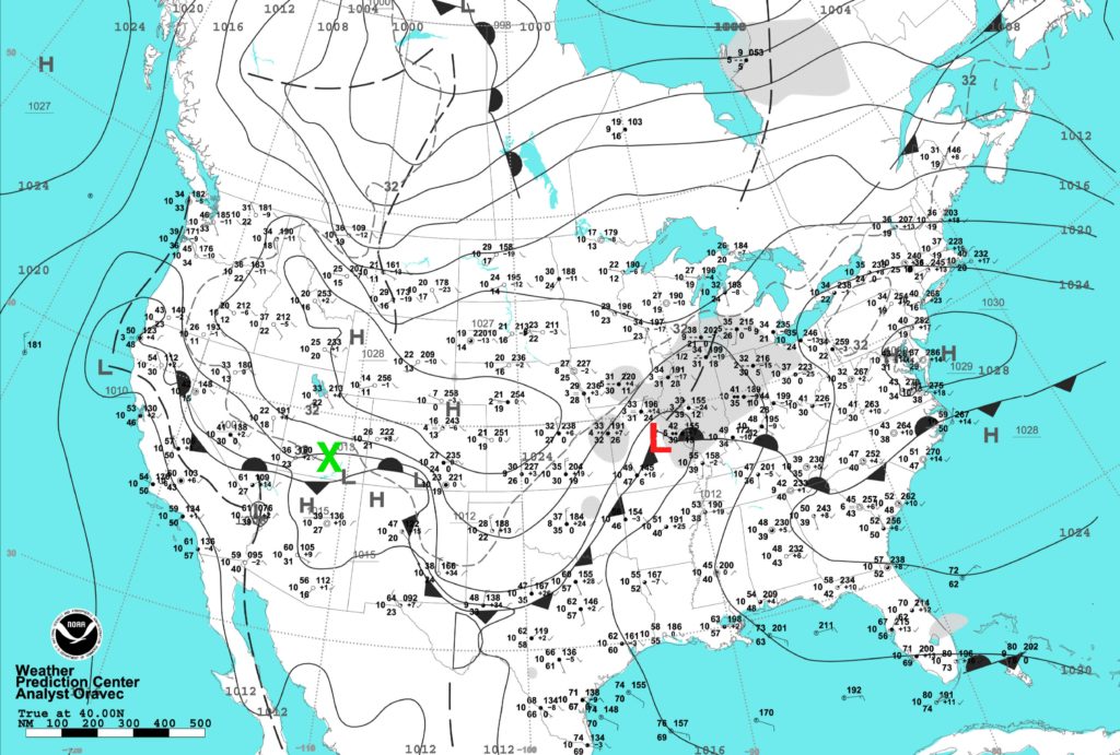
Figure 4.11. Surface weather map and station weather for Friday April 17, 2020 at 7:00 EST or 11:00 UTC (Z). Map Source: National Oceanic and Atmospheric Administration, Weather Prediction Center, Daily Weather Map website.
3.1) What is the approximate atmospheric pressure of the storm’s low center? Note that this value is usually found on the synoptic map in a font smaller than the one used to identify isobars – look below and to the right of the L.
3.2) What type of front is found south-southwest of storm’s low pressure center?
A Stationary front.
B Occluded front.
C Warm front.
D Cold front.
3.3) The surface air just east of the front mentioned in question 3.2 has temperatures roughly between
A 20 to 30 °F.
B 30 to 50 °F.
C 50 to 62°F.
3.4) The surface air just west of the front mentioned in question 3.3 has temperatures roughly between
A 20 to 30 °F.
B 30 to 50 °F.
C 50 to 62 °F.
3.5) What type of front is found east of storm’s low pressure center?
A Stationary front.
B Occluded front.
C Warm front.
D Cold front.
3.6) The surface winds just south of the front mentioned in question 3.5 are generally coming from the
A north.
B south.
C east.
D west.
3.7) The surface winds just north of the front mentioned in question 3.5 are generally coming from the
A north.
B south.
C east.
D west.
3.8) Grey shading on the synoptic weather map indicates areas where precipitation is occurring. What type of precipitation is associated (type and rate) with the mid-latitude cyclone? Where is it falling relative to the storm system?
3.9) How far has the storm travel in the last 24 hours? Note the green X shows the position of the low center 24 hours prior.
A About 400 nautical miles or 720 kilometers.
B About 800 nautical miles or 1440 kilometers.
C About 1200 nautical miles or 2160 kilometers.
3.10) What direction has the storm travel in the last 24 hours?
A North.
B East.
C South.
QUESTION 4
On the April 18, 2020 surface weather map, the low pressure center of a mid-latitude cyclone (red L) is now on the coastline of northeastern United States (Figure 4.12). The questions that follow are related to this storm system.
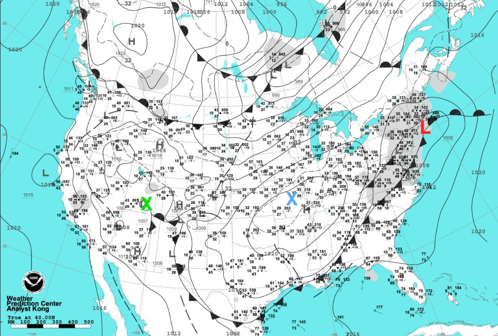
Figure 4.12. Surface weather map and station weather for Saturday April 18, 2020 at 7:00 EST or 11:00 UTC (Z). Map Source:National Oceanic and Atmospheric Administration, Weather Prediction Center, Daily Weather Map website.
4.1) What is the approximate atmospheric pressure of the storm’s low center? Note that this value is usually found on the synoptic map in a font smaller than the one used to identify isobars – look to the right of the L.
4.2) How far has the storm travel in the last 24 hours? Note the blue X shows the position of the low center 24 hours prior.
A About 400 nautical miles or 720 kilometers.
B About 800 nautical miles or 1440 kilometers.
C About 1200 nautical miles or 2160 kilometers.
4.3) How has the weather of the area south of the storm’s previous location 24 hours ago changed in terms of precipitation, temperature, atmospheric pressure, and cloud cover?
Students will write their responses here…
4.4) The air southeast of the cold front would most likely represent what type of air mass?
A Maritime polar.
B Maritime tropical.
C Continental tropical.
D Continental polar.
4.5) The air northwest of the cold front would most likely represent what type of air mass?
A Maritime polar.
B Maritime tropical.
C Continental tropical.
D Continental polar.
QUESTION 5
Examine the following two animations available on YouTube. These animations show the weather conditions that occurred in southern Canada, the USA, and northern Mexico for a 48-hour period from February 16th to February 18th, 2008.
One video shows surface air temperatures (°F), surface air pressure (isobars in mb), and centers of low and high pressure. The opening frames of this video display a mid-latitude cyclone located in the south-central USA. By the end of this video, this weather system moves in a northeasterly direction with it now being located in northern Quebec, Canada.
Video – Surface Temperature (°F) and Surface Air Pressure (mb), February 16 to 18, 2008
The second video displays GOES satellite infrared (IR) imagery combined with surface air pressure measurements. The infrared satellite images show information associated with the temperature of clouds and the Earth’s surface. Ground surfaces vary in shade from light grey to dark grey depending on the time of day. Ground surfaces become dark grey when incoming sunlight is converted into heat which in turn produces a higher surface emission of longwave radiation. After sunset, ground surfaces become lighter in tone as they cool off and their emission of infrared energy declines. The generally much colder cloud surfaces have a tone that varies from light grey to white. The white tone represents cold temperatures and the lowest emission of infrared radiation in the satellite image.
Video – Clouds and Surface Air Pressure (mb), February 16 to 18, 2008
Answer the following questions related to the two videos shown above. You will need the file Lab4_Question_5_Map.pdf found below to answer the first two questions.
5.1) On February 16th at 22 Z there is a low pressure center located in the south-eastern corner of Colorado. Follow the development of this low pressure center into a mid-latitude cyclone in both animations. Using the map given plot the location of the low pressure center on February 16th at 22 Z and February 18th at 22 Z. Draw a line between these points that traces the path taken by the mid-latitude cyclone. Submit this map to your teaching assistant. Estimate how far the storm system traveled in two days. Show your work.
5.2) Calculate the cyclone’s speed of travel in kilometers per hour. Show your work. Note that speed is equal to the distance traveled divided by the time, or duration, of travel.
5.3) Determine the surface air pressure (in millibars) of the cyclone’s low pressure center on February 16th at 22 Z.
5.4) Determine the surface air pressure (in millibars) of the cyclone’s low pressure center on February 18th at 22 Z.
5.5) According to the last two questions, did the storm intensify and become stronger? What happened to its central pressure? How would this influence wind flow? Explain.
5.6) Describe the temperature characteristics of air in the region slightly southeast of the mid-latitude cyclone’s low pressure center. How do the characteristics of this air (temperature and pressure) change after the cyclone leaves this area? Explain.
QUESTION 6
Meteorologists use General Circulation Models (GCMs) routinely to produce weather forecasts at regular intervals. Such forecasts are usually made up to seven days into the future, usually at either 3 or 6 hour intervals. The accuracy of these predictions is normally very high for about 3 days. After this threshold, accuracy declines steadily with time because of the difficulty of modeling the inherent chaotic behavior of many atmospheric processes.
We can access weather forecasts from government organizations like NOAA’s (National Oceanic and Atmospheric Administration) Weather Prediction Center website or Environment and Climate Change Canada‘s Weather Information website. Weather forecasts are also available from a variety of companies and non-governmental organizations. This is possible because current weather data and climate model-produced forecasts are made freely available through the World Meteorological Organization.
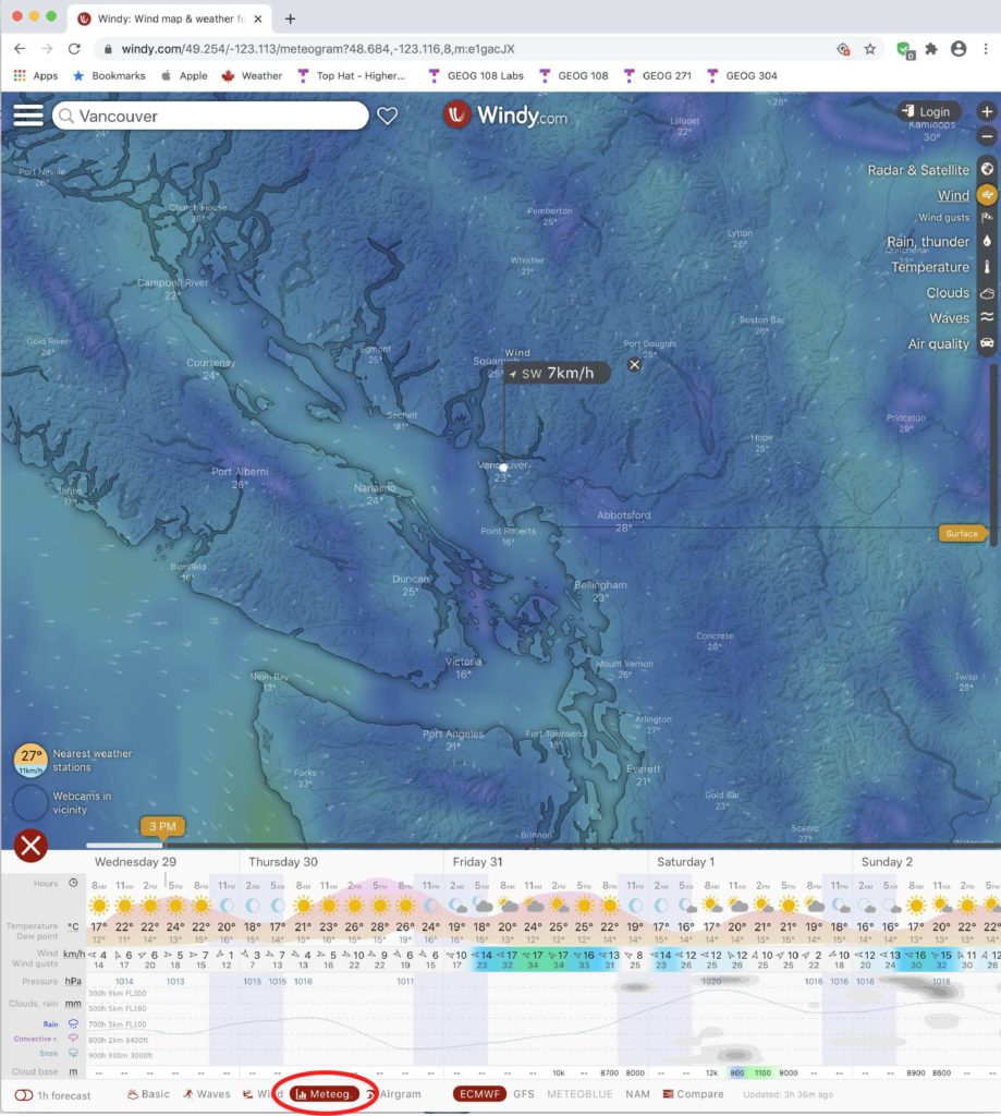
One website that offers an exceptional graphic interface for viewing prevailing weather conditions and future forecasts from local to the global scale is Windy.com. Windy is also available as an App that runs on smartphones, iPads, and other tablet computers. The image below shows Windy.com’s opening screen after I searched for Vancouver, British Columbia. The map window shows wind data (direction and speed). Along the bottom of the wind map window is a forecast window describing the first 5 days of a 7-day forecast, with each day segmented into 3-hour intervals (2 am, 5 am, 8 am, 11 am, 2 pm, 5 pm, and 11 pm), and the following “basic” weather information displayed: sky conditions, temperature (°C), rain (mm), wind speed (kph), wind gusts speed (kph), and wind direction.
![]()
In the next image, the “meteogram” option (red oval) was selected for the 7 day forecast output and the following weather data was made available: sky conditions, temperature (°C), dew point temperature (°C), wind speed (kph), wind gusts speed (kph), atmospheric pressure (hPa or mb), rain (mm), and cloud base (m).
Running down the right side is a series of buttons that control access to the weather data window in windy.com. The next image shows the Humidity (relative humidity) layer turned on in the map window. The Legend for this data layer is located in the bottom right-hand corner. It suggests the surface air over water bodies has a relative humidity of around 80-90%, while the air over land has a humidity of about 30-50%.
![]()
6.1) Produce a 24-hour forecast 3 days into the future for Winnipeg using Windy.com. Note the date of this forecast. Provide information on maximum and minimum temperature, dew point temperature, precipitation, wind speed and direction, atmospheric pressure, and sky conditions.
IMAGE CREDITS
Figure 4.1: Image Copyright Michael Pidwirny.
Figure 4.2: Image Copyright Michael Pidwirny.
Figure 4.3: Image Copyright Michael Pidwirny.
Figure 4.4: Image Copyright Michael Pidwirny.
Figure 4.5: Image Copyright Michael Pidwirny.
Figure 4.6: Image Source: National Oceanic and Atmospheric Administration, Weather Prediction Center, Daily Weather Map website. Public Domain.
Figure 4.7: Image Source: National Oceanic and Atmospheric Administration, Weather Prediction Center, Historical Archive of North American Analyses Webpage. Public Domain.
Figure 4.8: Image Source: National Oceanic and Atmospheric Administration, Weather Prediction Center, Historical Archive of North American Analyses Webpage. Public Domain.
Figure 4.9: Image Copyright Michael Pidwirny.
Figure 4.10: Image Source: National Oceanic and Atmospheric Administration, Weather Prediction Center, Daily Weather Map website. Public Domain.
Figure 4.11: Image Source: National Oceanic and Atmospheric Administration, Weather Prediction Center, Daily Weather Map website. Public Domain.
Figure 4.12: Image Source: National Oceanic and Atmospheric Administration, Weather Prediction Center, Daily Weather Map website. Public Domain.
QUESTION ANSWER SHEET
FIGURES AND TABLES – PDF FILES
This Laboratory Exercise is Licensed Under Attribution-NonCommercial-NoDerivatives 4.0 International (CC BY-NC-ND 4.0).
Updated April 26, 2021
A large body of air whose temperature and humidity characteristics remain relatively constant over a horizontal distance of hundreds to thousands of kilometers (miles). Air masses develop their climatic characteristics by remaining stationary over a source region for many days. Air masses are classified according to their temperature and humidity characteristics.
Region on the Earth where air masses originate and come to possess their particular moisture and temperature characteristics.
Air mass that forms over extensive ocean areas of the middle to high latitudes. Around North America, these air mass systems form over the Atlantic Ocean and Pacific Ocean at the middle latitudes. Maritime Polar air masses are mild and humid in summer and cool and humid in winter. In the Northern Hemisphere, maritime polar air masses are normally unstable during the winter. In the summer, atmospheric stability depends on the position of the air mass relative to a continent. Around North America, Maritime Polar air masses found over the Atlantic are stable in summer, while Pacific systems tend to be unstable.
Air mass that forms over extensive landmass areas of middle to high latitudes. In North America, these systems form over northern Canada. Continental Polar air masses are cold and very dry in the winter and cool and dry in the summer. These air masses are also atmospherically stable in all seasons. On weather maps, the symbol cP is used to identify a Continental Polar air mass.
Air mass that forms over extensive ocean areas of the low latitudes. Around North America, these systems form over the Gulf of Mexico and the eastern tropical Pacific. Maritime Tropical air masses are warm and humid in both winter and summer. In the Northern Hemisphere, maritime tropical air masses can normally be stable during the whole year if they have form just west of a continent. If they form just east of a continent, these air masses will be unstable in both winter and summer.
Air mass that forms over extensive landmasses areas of the low latitudes. In North America, these systems form over the southwestern United States and northern Mexico. Continental Tropical air masses are warm and dry in the winter and hot and dry in the summer. These air masses are also generally unstable in the winter but stable in the summer. On weather maps, the symbol cT is used to identify a Continental Tropical air mass.
Air mass that forms over extensive landmass areas in the high latitudes of the Northern Hemisphere. These air mass systems form only in winter over Greenland, northern Canada, northern Siberia, and the Arctic Basin. Continental Arctic air masses are very cold, extremely dry, and very stable. On weather maps, the symbol cA is used to identify a Continental Arctic air mass.
A transition area that exists between two air masses with different air temperature and/or humidity characteristics. Differences in air temperature and/or humidity causes the air mass with lower air density to be pushed over the denser air mass. This process is known as frontal lifting and can result in the development of clouds and precipitation.
A transition zone found between air masses with different air densities and weather characteristics.
Lifting of a warmer or less dense air mass by a colder or more dense air mass at a frontal transitional zone. This process causes the water vapor in the warmer air to cool, and then condense or freeze, forming clouds and precipitation.
Cyclonic storm that forms primarily in the middle latitudes. The formation of these storms is triggered by the development of troughs in the polar jet stream. These storms also contain warm, cold, and occluded fronts. Atmospheric pressure in their center can get as low as 970 millibars. Also called wave cyclones or frontal cyclones.
Relatively fast uniform winds concentrated within the upper atmosphere in a narrow band. Several jet streams have been identified in the atmosphere. The polar jet stream exists in the mid-latitudes at an altitude of approximately 10 kilometers (6.2 miles). This jet stream flows from west to east at average speeds, depending on the time of year, between 110 to 185 kilometers per hour (68 to 115 miles per hour). Another strong jet stream occurs above the Subtropical Highs at an altitude of 13 kilometers (8.1 miles). This jet stream is commonly called the subtropical jet stream. The subtropical jet stream's winds are not as strong as the polar jet stream.
Weather front located typically in the mid-latitudes that separates arctic and polar air masses from tropical air masses. Along the polar front we get the development of the mid-latitude cyclone. Above the polar front exists the polar jet stream.
A transition zone in the atmosphere where an advancing cold air mass displaces a warm air mass. A shallow zone of cloud development and heavy precipitation usually occurs behind of the front. Compare with occluded front and warm front. Normally associated with mid-latitude cyclones.
A transition zone in the atmosphere where an advancing warm air mass displaces a cold air mass. A wide band of cloud development and light precipitation usually occurs ahead of the front. Compare with cold front and occluded front. Associated with mid-latitude cyclones.
Is any aqueous deposit, in liquid or solid form, that develops in a saturated atmosphere (relative humidity equals 100%) and falls to the ground generally from clouds. Most clouds, however, do not produce precipitation. In many clouds, water droplets and ice crystals are too small to overcome natural updrafts found in the atmosphere. As a result, the tiny water droplets and ice crystals remain suspended in the atmosphere as clouds. Some forms of precipitation include rain, snow, drizzle, hail, ice pellets, and snow pellets.
A well developed vertical cloud that often displays a top shaped like an anvil. Cumulonimbus clouds are very dense with condensed water droplets and deposited ice crystals. Common weather associated with this cloud includes: strong winds; hail; lightning; tornadoes; thunder; and heavy rain. When this weather occurs these clouds are then officially called thunderstorms. These clouds can extend in altitude from a few hundred meters above the surface to more than 12,000 meters (39,400 feet).
This term is used to designate a thunderstorm that has reached a particular level of severity. This is an intense storm with frequent lightning and local wind gusts of 97 kph (60 mph), or hail that is 2 cm (3/4 of inch) in diameter or larger. Severe thunderstorms can also have tornadoes. In Canada, thunderstorms are also considered severe if their rainfall exceeds 50 millimeters (2 inches) in one hour, or 75 millimeters (3 inches) in three hours.
A dark gray low altitude cloud that produces continuous precipitation in the form of rain or snow. Found in an altitude range from the surface to 3,000 meters (9,840 feet).
Gray-looking middle altitude cloud that is composed of water droplets and ice crystals. Appears in the atmosphere as dense sheet-like layer. Can be recognized from stratus clouds by the fact that you can see the Sun through it. Found in an altitude range from 2,000 to 8,000 meters (6,500 to 26,250 feet).
High altitude sheet-like cloud composed of ice crystals. These thin clouds often cover an extensive area of the sky. Found in an altitude range from 5,000 to 18,000 meters (16,400 to 59,050 feet).
The process of cyclone formation, maturation, and death. Associated with tropical storms, hurricanes, and mid-latitude cyclones.
A transition zone in the atmosphere where there is little movement of opposing air masses and where winds blow towards the front from opposite directions.
A transition zone in the atmosphere where an advancing cold air mass sandwiches a warm air mass between another cold air mass pushing the warm air into the upper atmosphere. Cloud development and precipitation usually occurs above of the occluded front. Compare with cold front and warm front. Associated with mid-latitude cyclones.
Map that displays the condition of the physical state of the atmosphere and its circulation at a specific time over a region of the Earth. Weather maps can display the values of many common meteorological variables measured at weather stations.
The mean solar time of the meridian at the Prime Meridian. Universal Time replaced the time standard known as Greenwich Mean Time in 1928. Universal Time is commonly used to denote solar time.
Is the temperature at which water vapor saturates from an air mass into liquid forming rain or dew. Dew point normally occurs when a mass of air has a relative humidity of 100% and temperatures are above 0°C. If the dew point is below freezing, it is referred to as the frost point.
The speed at which a wind is blowing. Usually measured in meters per second, kilometers per hour, feet per second, or miles per hour.
The direction from which a wind blows. Usually measured in cardinal and intercardinal directions or in degrees azimuth.
The weight of the atmosphere on a surface. At sea level, the average atmospheric pressure is 1013.25 millibars (29.92 inches of mercury). Atmospheric pressure can be measured by a device called a barometer.
