6 Bond Graph Models for Complex Mechanical Systems
6.1 Overview
In the previous chapters, we established concepts such as the basic elements of bond graph method and the algorithm for building BG models. We now continue with more worked-out examples for selected complex mechanical systems. These systems may have many components, involve many degrees of freedom, and exhibit translational and rotational motions in one-dimensional (1D) or two-dimensional (2D) space. So far, we have used translational mechanical systems and demonstrated how to build their related BG models (see chapters 4 and 5). In this chapter, we expand the discussion to rotational mechanical systems with rotational and/or 2D/plane rigid-body motions, including their related BG model examples. First, we establish the theories and related equations and then use those for building the BG models.
6.2 Mechanical Systems—Rotational
A mechanical system may consist of rotational components, e.g., shafts, discs, gears, pulleys, and levers. The generalized BG elements and relations apply to the motion of rotational components in a similar way that the translational motion was treated; i.e., they are analogous (see Table 3‑1). In other words, rotation angle  is equivalent to the generalized displacement
  , angular velocity
  to the flow
  , and torque
  to the effort
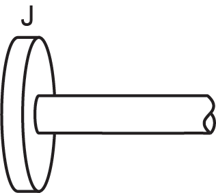
  . The polar moment of inertia
  is represented by
  -element, the shaft by
  -element, and bearing by
  -element. The generalized momentum is the integral of with respect to time. Therefore, we can write

where  is the rotational momentum or so-called angular momentum. Using the constitutive relations, for an -element we have
  or
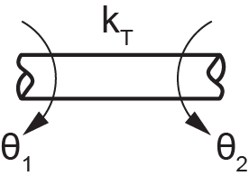
or  , for a -element we have
  or,
or,  where
where  represents the torsional compliance or inverse of torsional stiffness
  ,
,  . Similarly, for an -element we have
  or
or  where
where  is the friction of the torsional bearing. The energy associated with storage elements can be written using Equations (3.7) and (3.8), or for elements and , as
  and
and  , respectively. One advantage of bond graph method is its analogous applicability to different domains using the common constitutive relations, as described above for rotational motion.
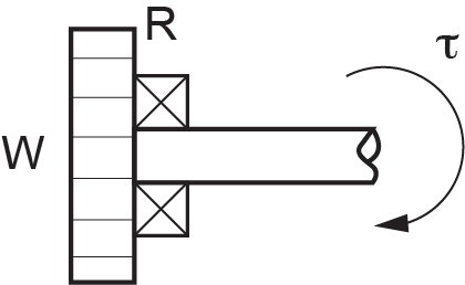
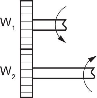
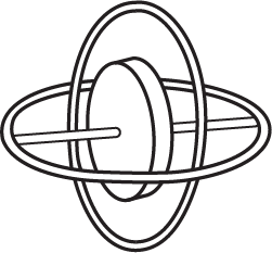
Table 6‑1 shows typical rotational components.
| -element (bearings) |
-element (shaft) |
-element (disc) |
 -element -element(gears) |
 -element -element(gyrator) |
 |
 |
 |
 |
 |
6.3 Mechanical Systems—Two-Dimensional Rigid Plane Motion
The components of mechanical systems that we considered so far are assumed as point masses. In other words, they are point elements but can have motions either in translation and/or rotation. However, two-dimensional components such as rigid plates, car chassis, and thin rods can have relative 2D motion and cannot be treated as point elements.
In general, a 3D solid component/body has six degrees of freedom; i.e., its centre of mass can move in three translational directions and through three associated rotational angles. In many mechanical systems, however, we can assume components as two-dimensional planes with negligible deformations, or as 2D rigid bodies having three degrees of freedom: two in-plane translations and one rotation about the perpendicular axis to the plane of motion.
Building a BG model requires transforming the velocities and angular velocities associated with the rigid plane and making them available to the contact points with other components of the system. For example, a car’s chassis moving forward on a wavy road may experience rotations like pitch and roll (i.e., rotations about the axes parallel to the ground) in addition to translational motion. Considering the chassis as a 2D rigid body, we need to know how the linear and angular velocities are transmitted to the suspensions connecting to it.
We present here an analysis of 2D rigid-body motion, with focus on applications to BG modelling. For further readings on this topic, consult with available references [13], [18], [20], [23].
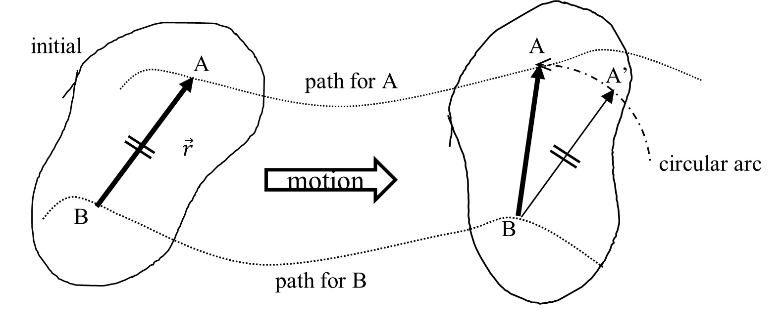
The general motion of a 2D rigid body can be decomposed into translation of the whole body and a rotation about a fixed point of the body. This is the result of the principle of superposition and can be shown using the geometry of the motion. As Figure 6‑1 shows, we assume a rigid body going through a planar motion with reference to a fixed coordinate system  . We identify a line/vector on the body connecting two arbitrarily selected points A and B, with point B taken as a reference, usually the centre of mass. We then capture a picture of the body at a later time,
  during its motion, and find out the line BA in its new orientation and position, as shown in the sketch on the right in Figure 6‑1. Since the body does not deform, the length of the line BA (or the magnitude of vector
  ) remains constant. Using this property, we can draw a circle with its centre at the new position of point B and radius of BA. Then, we draw the radial line BA’ parallel to the line BA at its initial position. To orient BA’ according to the new position of BA, we then rotate BA’ about point B through angle
  , where
  is the magnitude of the angular velocity vector of the rigid body, perpendicular to the plane of motion. Consequently, we can claim that original point A is translated (not rotated) by the velocity of point B,
  from its initial position to a new position A’ and subsequently rotated about point B by angle to orient in its final new position of point A. The initial position of point A is arbitrarily selected; therefore, the argument equally applies to all points of the rigid body.
Mathematically, we can write  . The relative velocity
  is the tangential velocity due to rotation and can be written as
  . Therefore,
  . Therefore, we can write the velocity components of point A resulted from rigid-body motion as
(6.1) 
But  and
and  where, is the angle between vector
  and positive direction of
  -axis. After substituting, we get
(6.2) 
We can use Equations (6.2) for large rotations. However, for small rotations (i.e.,  ), we can linearize these relations by substituting for
  and
and  , or
, or
(6.3) 
For example, for a car chassis, the front and rear ends are moving with the same speed as that of the centre of mass, and their velocities in the vertical direction are the algebraic sum of the vertical speed and that of due to the pitch rotation (i.e., rotation about the axis parallel to the ground and perpendicular to the direction of the motion). See the example in section 6.7.
In the following sections, we present examples of several mechanical systems along with their BG models.
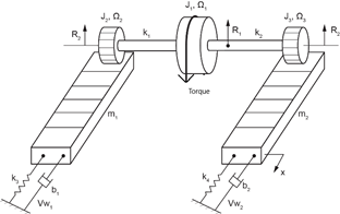
6.4 Example: Gear-Shaft Mechanical System—Rotational
The sketch in Figure 6‑2 shows a system composed of four gears, three shafts, six bearings, and two discs.
- Build the BG model for this system, including bearings. Use 20-sim.
- Identify derivative causalities and the related elements. Discuss the reasoning and how to remove the derivative causalities.
- Remove all bearings from the model and perform some analysis using the data provided.
For gears, use velocity ratio,  equal to the inverse ratio of the number of teeth,
  or gears’ diameters,
  given by
  . Angular velocity of gears is represented by the symbol
  . System data is given in Table 6‑2.

Solution:
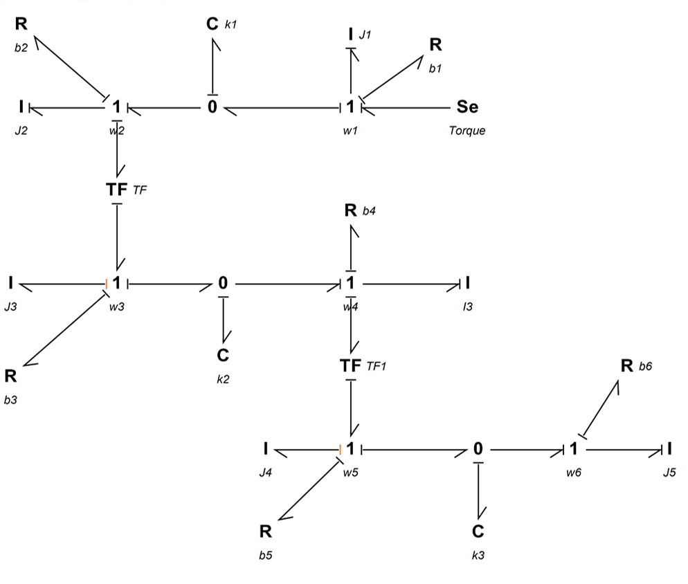
This system has six distinct angular velocities related to gears and discs. The torsional shafts are potential energy storages, and the torsional inertia are kinetic energy storages. The BG elements required are , , ,  ,
,  , and 1- and 0-junctions.
The following video shows how to build and run the model for this example in 20-sim.
The resulted BG models are shown in Figure 6‑3 and Figure 6‑4.
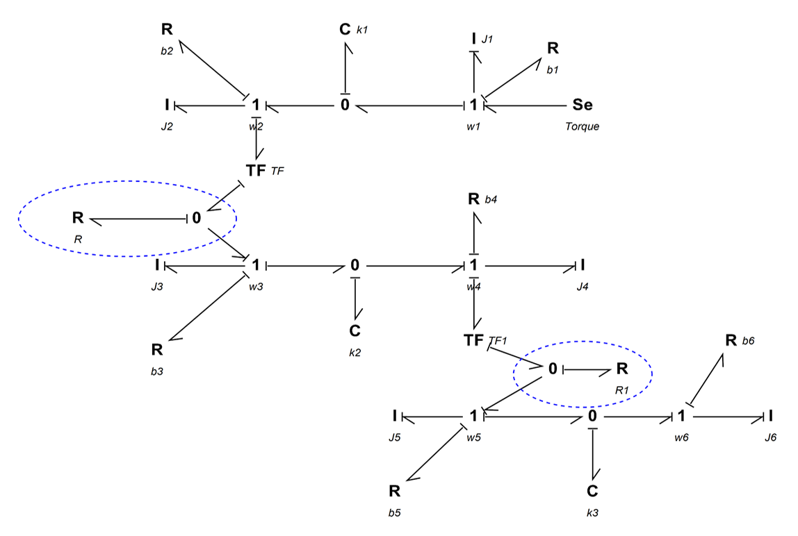
6.5 Example: Double Rack-and-Pinion Mechanical System—Rotational
Figure 6‑5 shows a double rack-and-pinion mechanical system. Build a BG model for this system using 20-sim. A torque is applied on the disc connected to the two shafts.
The following video shows how to build and run the model for this example in 20-sim.
Figure 6‑6 shows the BG model for this system.
6.6 Example: Mass-Spring-Damper System on an Inclined Plane—Translational
Figure 6‑7 show a mass-spring-damper system on an inclined plane. Build a BG model for this system using 20-sim. Build a BG model for this system using 20-sim.
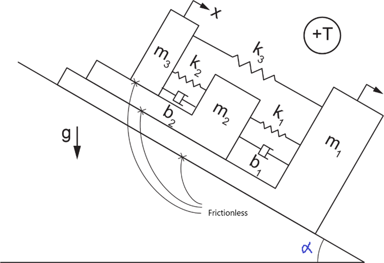
The following video shows how to build and run the model for this example in 20-sim.
Figure 6‑8 shows the BG model for this system.
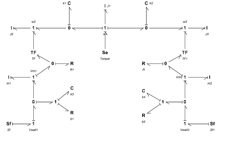
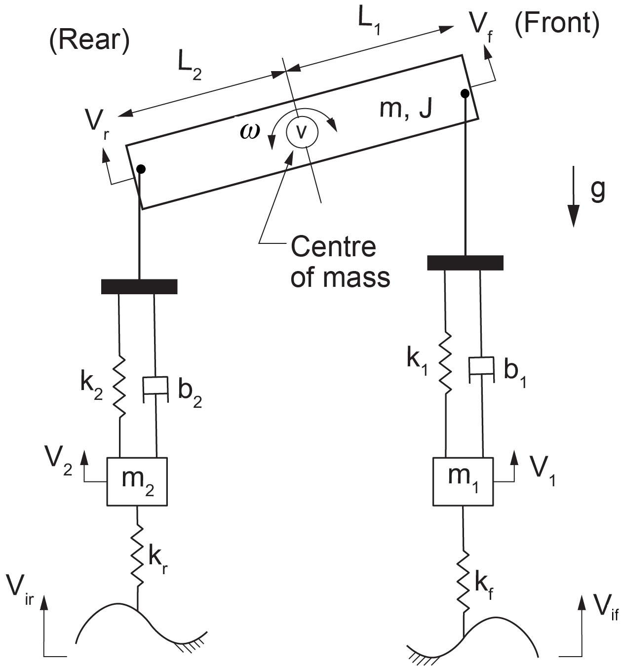
6.7 Example: 2D Rigid-Body Motion—Half-Car Model
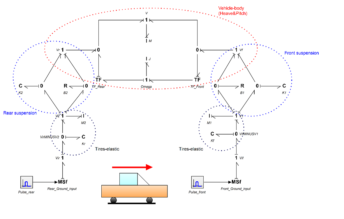
In this example, we demonstrate how to build a BG model for a half-car model as shown in Figure 6‑9. The chassis of the car is modelled as a rigid body with two degrees of freedom. The vertical displacement of the centre of mass is the heave, and its angular velocity is the pitch rate. In the BG model, transformer elements are used to transfer the front and rear velocities to the corresponding connecting points between the suspensions and the chassis. The suspension are modelled as spring-dampers and the tires as mass-spring subsystems.
Below are two videos (parts 1 and 2) showing how to build and run the model for this example in 20-sim, including the implementation of the BG transformer element and the setup of the equation model.
Watch the videos and practice building the model on your own, with modified parameters and input signals.
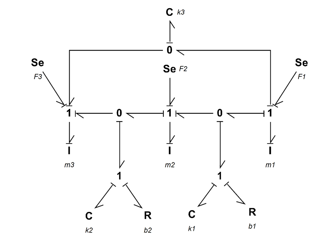
Figure 6‑10 shows the corresponding BG model. The compression force is considered to be positive.
6.8 Example: Mass-Spring-Damper System Connected to a Massless Lever
In this example, we demonstrate how to build a BG model for the mechanical system shown in Figure 6‑11. The lever is represented with a -element.
Below are two videos (parts 1 and 2) showing how to build and run the model for this example in 20-sim, including the implementation of the BG transformer element and the setup of the equation model.
6.9 Example: Mass-Spring-Damper System Connected to a Lever
For this example we discuss and demonstrate how to build a BG model for the mechanical system as shown in Figure 6‑12. The lever is represented with a -element.
Below are two videos (parts 1 and 2) showing how to build and run the model for this example in 20-sim, including the implementation of the BG transformer element and the setup of the equation model.
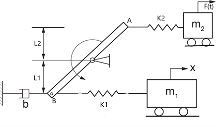
6.10 Example: Inclined Lever and Mass-Spring-Damper System
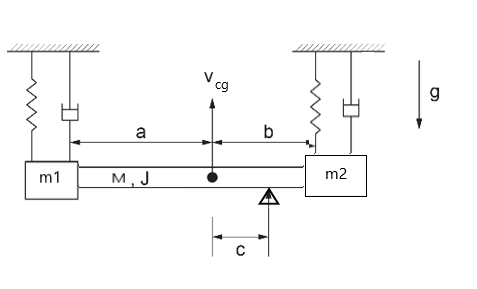
In this example, we demonstrate how to build a BG model for a mechanical system consisting of two moving masses attached to a rod, as shown in Figure 6‑13. The rod can rotate as a lever and is represented with a -element.
The following video shows how to build and run the model for this example in 20-sim.
6.11 Example: A Pulley-Mass-Spring System
In this example, we demonstrate how to build a BG model for a mechanical system consisting of two pulleys and three masses, as shown in Figure 6‑14.
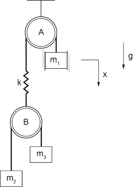
The video below shows how to build and run the model for this example in 20-sim.
Exercise Problems For Chapter 6
Exercises
- Repeat the BG model using 20-sim for the half-car system given in section 6.7, considering following cases, inclusively and suggested data:
 ,
,  (kg),
(kg),  ,
,  (m),
(m),  (kg.m2/rad),
  ,
,  ,
,  (kN/m),
  ,
,  (kN.s/m)
- ground velocity signal as a pulse signal with start time at 1.5 sec., stop time at 3 sec., and amplitude of 10 cm/s
- ground velocity signal as a step signal with start time at 1.5 sec. and amplitude of 10 cm/s
- ground velocity signals such that the car hits a trapezoidal-shaped bump at 1.5s of time, reaches the top of the ramp at 3.5s, stays on top of the plateaued bump for 2s, and comes back to ground level with a similar slope. The amplitude of the velocity signals is 10 cm/s.
- ground velocity signal as a pulse wave signal with interval of 1 sec., pulse length of 0.1 sec., and amplitude of 5 cm.
- For all inputs, graph the displacements of the tires and the heave and pitch of the car chassis.
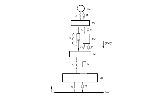
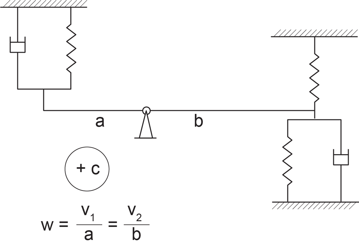
- Using 20-sim, build a BG model for the mechanical system shown in the sketch below. Use the data to graph the displacement of the mass
 ,
,  , and spring
  . Consider the floor velocity input as a pulse signal with start time of 3 sec., stop time of 4.5 sec., and amplitude of 10 cm. Compression forces are considered to be positive (+C). Gravity direction and positive displacements are shown in the sketch.
| Masses (kg) |  |
 |
 |
 |
 |
— |
| Springs (N/m) |  |
 |
 |
 |
 |
 |
| Dampers (N.s/m) |  |
 |
 |
 |
 |
 |