2 Lagrangian Mechanics
2.1 Overview
In general, it is easier to perform engineering/technical calculations using a scalar quantity rather than a tensor/vector type quantity, mainly because a vector’s components depend on the selected coordinates system, and hence, more quantities to deal with. This was the main motivation for Joseph-Louis Lagrange (1736–1813), [7], [8] to start looking into the Newtonian mechanics close to a century after Newton developed his laws. Consequently, Lagrange developed a new formulation, so-called Lagrangian mechanics (1788).
Lagrange’s approach has advantages over that of Newton’s, specifically for analyzing complex multi-domain, multi-component systems. Lagrange’s approach releases us from having to consider a single inertia coordinates system and inter-component constraint forces. In addition, Langrangian method is faster and more efficient in terms of computation time and effort required to analyze and model engineering systems.
In Newtonian mechanics, a local condition, e.g., initial position and velocity (or momentum), is required for calculating the future states of a system. Using Newton’s law of motion, for a system or components of a system, the sum of forces (both applied,  and constrained/internal,
  ), is equal to the time rate of change of the momentum,
  .
.
(2.1) 
In order to identify the constraints, we usually isolate the components one by one from the rest of the system, while keeping the related dynamical equilibrium intact. This operation gives us the free-body diagram of each desired component, useful for analyzing the system’s motion dynamics and calculating inter-component constraint forces. However, in the Lagrangian approach, we consider a quantity that is like energy in dimension, the Lagrangian  , and use a set of partial differential equations (PDEs)—Euler-Lagrange or Lagrange’s equations— to analyze the system dynamics.
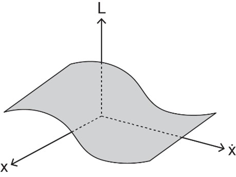
The latter is much more effective approach for analyzing the systems with many degrees of freedom and for dealing with multi-domain systems. In general, L is a function of coordinates considered and their time derivatives and, as well, could explicitly depend on time. For example, in a one-dimensional system, with designated coordinate x, the Lagrangian is written as  We can visualize as the topography of a surface represented by as a function of
  and
and  , as shown in Figure 2-1. This surface can vary with time, hence explicit dependence of on time, or it could be stationary. An example of the former is the motion of a mass particle on the surface of a moving sphere. Similarly, the Lagrangian of such a system is stationary if the sphere is not moving. The visualization presented in reference [9] may help readers with understanding Lagrangian surface.
 space
spaceThe foundation of Lagrangian mechanics rests on the principle of stationary action integral (also referred to as Hamilton’s principle) . This principle simply states that a system’s motion from a given state to another is such that a specific quantity (i.e., the system’s Lagrangian function) related to its motion is extremized (i.e., minimized or maximized); hence, the value of its integral (i.e., the action integral,  ) remains invariant [10].
 to
to  is such that the action integral has a stationary value for the actual path of the motion
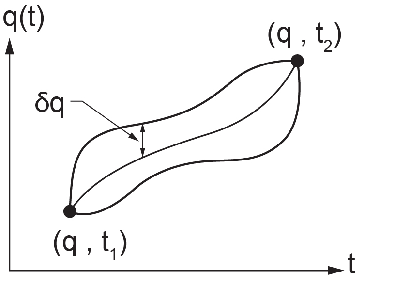
In other words, among all possible paths available for the motion of the system to go through, there exists one specific path that minimizes/maximizes (for most systems minimizes; hence, this is also referred to a principle of least action) the integral of the corresponding Lagrangian with respect to time. Mathematically, the stationary action integral can be stated as
(2.2) ![\begin{equation*} \delta \mathcal{A} = \delta \left[ \int_{t_1}^{t_2} L(x,\dot x, t)dt \right] = 0 \end{equation*}](https://pressbooks.bccampus.ca/engineeringsystems/wp-content/ql-cache/quicklatex.com-344834e0991f50a49772686f4b0d25d2_l3.png "Rendered by QuickLaTeX.com")
Using calculus of variations [11], [12], [13] and Equation (2.2) it can be shown (see section 2.5) that L should satisfy Lagrange’s equation, or
(2.3) 
where L is defined as  , with
  being the kinetic energy and
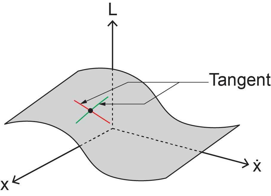
  the potential energy functions. With reference to Figure 2-1,
  is the slope at a selected point on the curve at the cross-section of surface and a plane parallel to -plane at desired , and
  is the rate of change in the slope at the same selected point on the curve at the cross-section of a plane parallel to -plane drawn from and including the selected point the same point. In other words, we draw two planes parallel to the and planes and equate their corresponding slopes at their intersectional point. Therefore, for a stationary point, these two quantities should be equal, as given by Euler’s equation (2.3). This is shown in the following sketch, see Figure 2-2.
By working out a simple example, we show that the Lagrangian approach is equivalent to the Newtonian approach in terms of the system’s equation of motion.
2.2 Example: A Mass-Spring System
For this example, we show that Equation (2.3) gives the same results as that of Newton’s law of motion when applied to a simple mass-spring system, as sketched in Figure 2-3.
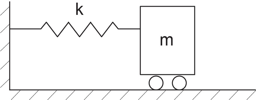
The kinetic energy for the mass  is
is  and the spring potential energy (i.e. stored elastic energy) with the spring constant k is
  . Therefore, using Equation (2.3), we get
 ![\dfrac{d}{dt} \left[ \dfrac{\partial}{\partial \dot x} \left(\dfrac{1}{2}m\dot x^2 - \dfrac{1}{2}kx^2 \right) \right] - \dfrac{\partial}{\partial x} \left(\dfrac{1}{2}m \dot x^2 - \dfrac{1}{2}kx^2 \right) = 0](https://pressbooks.bccampus.ca/engineeringsystems/wp-content/ql-cache/quicklatex.com-d95c10fd3e54c3ef6fd35149898e4bba_l3.png "Rendered by QuickLaTeX.com") , or
, or  . Note that for this analysis we did not need to consider the free-body diagram of mass nor the spring force as the constraining force acting on it; rather, we used the scalar quantity
  . However, the assumption of having a potential function from which we can calculate the spring force is required (i.e.,
  ), see section 2.7.
In the following sections we expand on the Lagrangian method for discrete systems with related derivation, constraints and definitions for generalized coordinates, forces, and momenta.
2.3 Lagrange’s Equations for a Mass System in 3D Space
We consider a particle with mass in a 3D space  , Cartesian system. By definition, the Lagrangian function is written as
  . We have assumed that the potential energy function is only a function of the space coordinates, so-called holonomic system. We now form two sets of derivatives
  and
and  of the Lagrangian function
  . Therefore, e.g., in 1D space, we have
  and
and  . Hence
  is a conservative force (see section 2.7). Now, using Newton’s second law, we can write the equation of motion, its -component, as
  or
or  and
and  Therefore,
  . Similar derivation can be performed for
  and
and  components of the equation of motion. Therefore, we get the Euler-Lagrange equations
(2.4) 
The motion of the particle could be considered, in principle, in another coordinate system, e.g., a cylindrical or spherical system, as well. Therefore, we can define a set of coordinates  to represent arbitrary coordinate systems, including Cartesian or curvilinear, and write Equation (2.4) in terms of
  , as well, for generality.
2.4 Generalized Coordinates, Momenta, and Forces
As mentioned previously, one of the advantages of Lagrangian method is that we do not require consideration of the constrained forces. Therefore, we can include only those coordinates that correspond to the degrees of freedom related to a system. This consideration leads us to the concept of generalized coordinates, which is used in Lagrangian mechanics instead of inertia coordinates used in the Newtonian mechanics.
We now define the generalized coordinates. First, we expand the system discussed in section 2.3 to include  number of particles that move in
  coordinate space, or
  . However, in a real-world system we can have restrictions imposed on the system’s motion; hence, some of the coordinates are constrained and do not vary independently. For example, a particle moving in a plane
  is constrained to move in -direction
  . Or, the mass bob of a pendulum moving in
  plane is restricted to move out of -plane and if the pendulum rod has a fixed length, then only coordinate
  varies during its motion. To capture these constraints, it is common and convenient to define generalized coordinates. Assume that for a coordinates system we have
  number of constraints. Therefore, the number of independent coordinates defining the motion is
  . By definition, for holonomic systems this is equal to the number of degrees of freedom [13]. Now we define the generalized coordinates as a subset of the original coordinates, with
  . Note that
  is the number of degrees of freedom which is equal to the number of generalized coordinates, and coordinates of the
  system are not necessarily the same as those of the , by one-to-one comparison.
For derivation of the equations of motion of a system, using Lagrangian approach, we can calculate  number of equations for the system, one by one, related to each generalized coordinate. We can also use the generalized coordinates to define the velocity-phase space, as the combined set of generalized coordinates and their corresponding time derivatives. Therefore, the Lagrangian, as a functional, reads
(2.5) 
Note that the time dependence of Lagrangian may be explicit for some systems and implicit for others and that the phase-space coordinates do not necessarily have the same units/dimensions. For example,  could be a displacement and
  an angle for a system like a pendulum with moving pivot point.
The fact that we can neglect the constrained coordinates in Lagrangian formulation is an advantage of this method over Newton’s because we don’t need to calculate the constrained “forces” in order to derive the equations of motion. Of course, the constrained forces can be calculated, if required, after having the solution to the system’s equations of motion.
Like the generalized coordinates, we also define associated generalized momenta and forces. As mentioned in the previous section, the definition of momentum in Lagrangian mechanics is more general than that of mass times the velocity. For example, it could be angular momentum, instead. Similarly, the definition of forces is not limited to mechanical forces; it can be applied, e.g., to voltage and temperature in electrical and thermal domains. Therefore, for each generalized coordinate we can define the corresponding generalized momentum and force. As given by Equation (2.6), we can write the generalized momenta and generalized force in terms of , as
(2.6) 
Section 2.7 discusses the topic of generalized force in terms of its types: conservative and non-conservative.
2.5 Hamilton’s Principle and Lagrange’s Equations
Hamilton’s principle, as given by Equation (2.2), is basically a mathematical expression of calculus of variations application for a system dynamical motion with the realization that Lagrangian functional is the function that should be extremized [12]. Therefore, Lagrange’s equations are resulted from the related calculations, naturally. This realization was first expressed by William Rowan Hamilton (1805-1865), [14], [11], [15].
Equation (2.4) can be written in terms of generalized coordinates, as
(2.7) 
Equation (2.7) shows that Lagrange’s equation is consequence of, and necessary for, making the action integral stationary. We assume that variation  results from variation in one of the arbitrarily selected coordinates,
  (dropping the subscript index for simplicity without losing the generality) while satisfying the fixed boundary conditions, or
  . Obviously, the same operation can be performed for all coordinates involved,
  .
.
 for an arbitrary
 Substituting Equation (2.7) into Equation (2.2), after dropping the subscript index and assuming  for simplicity, we get
![\begin{equation*} \delta \mathcal{A} = \delta \Big\{ \int_{t_1}^{t_2} \left[ \frac{d}{dt} \left( \frac{\partial L}{\partial \dot q} \right) - \frac{\partial L}{\partial q} \right] dt\Big\} = \Bigg\{ \int_{t_1}^{t_2} \delta \big\[\underbrace{\left[ \frac{d}{dt} \left( \frac{\partial L}{\partial \dot q} \right) - \frac{\partial L}{\partial q} \right]}_{L} \big\ dt \Bigg\} = 0 \end{equation*}](https://pressbooks.bccampus.ca/engineeringsystems/wp-content/ql-cache/quicklatex.com-46a4c7858d29f053da7696e5171c7e60_l3.png "Rendered by QuickLaTeX.com")
But  and the last term can be written as
  and hence,
 ![\delta L = \left[ \dfrac{\partial L}{\partial q} - \dfrac{d}{dt} \left(\dfrac{\partial L}{\partial \dot q} \right) \right] \delta q + \dfrac{d}{dt} \left( \dfrac{\partial L}{\partial \dot q} \delta q \right)](https://pressbooks.bccampus.ca/engineeringsystems/wp-content/ql-cache/quicklatex.com-2711aa9630f548aa98c44955112ff9b2_l3.png "Rendered by QuickLaTeX.com") .
.
Back substituting into action integral expression, we get ![\delta \mathcal{A} = \int_{t_1}^{t_2} \left[ \dfrac{\partial L}{\partial q} - \dfrac{d}{dt} \left( \dfrac{\partial L}{\partial \dot q} \right) \right] \delta q \: dt + \int_{t_1}^{t_2} \dfrac{d}{dt} \left( \dfrac{\partial L}{\partial \dot q} \delta q \right) dt = 0](https://pressbooks.bccampus.ca/engineeringsystems/wp-content/ql-cache/quicklatex.com-dbec2b1c54535b2f414ce9ab10b71a82_l3.png "Rendered by QuickLaTeX.com") .
.
But the last integral gives ![\int_{t_1}^{t_2} \dfrac{d}{dt} \left( \dfrac{\partial L}{\partial \dot q} \delta q \right) dt = \dfrac{\partial L}{\partial \dot q} \delta q \Big|_{t_1}^{t_2} = \dfrac{\partial L}{\partial \dot q} \bigg[ \underbrace{\delta q (t_2) - \delta q(t_1)}_{=0} \bigg] = 0](https://pressbooks.bccampus.ca/engineeringsystems/wp-content/ql-cache/quicklatex.com-15273469054b07de4ccf371eee47e001_l3.png "Rendered by QuickLaTeX.com") .
.
Therefore, we have ![\delta \mathcal{A} = \int_{t_1}^{t_2} \left[ \dfrac{\partial L}{\partial q} - \dfrac{d}{dt} \left( \dfrac{\partial L}{\partial \dot q} \right) \right] \delta q \: dt = 0](https://pressbooks.bccampus.ca/engineeringsystems/wp-content/ql-cache/quicklatex.com-3b0fc29a446a63dacc6223f5758cf0a2_l3.png "Rendered by QuickLaTeX.com") . Since is arbitrarily selected, the integrand should be equal to zero in order to have the value of the integral null, or
. Since is arbitrarily selected, the integrand should be equal to zero in order to have the value of the integral null, or  . This concludes the derivation of Lagrange’s equation using Hamilton’s principle. However, one can derive Lagrange’s equation in a more direct way using calculus of variations or virtual work principles, see [11], [13], [16].
So far, we have considered systems that do not involve energy dissipation. In practice, however, we require extra terms in Lagrange’s equation to account for friction existing in real-world systems. Therefore, we expand the discussion to include non-conservative forces, e.g., friction and dampers, and find the corresponding Lagrange equation, including related topics such as cyclic coordinates, symmetry, multi-domain, and higher-order systems, [8], [13], [17].
2.6 Cyclic Coordinates
From Equation (2.6), it can be shown that if Lagrangian function does not have explicit dependency on one of the coordinates, say  , among all , then the conjugate momentum
  is conserved. The proof is as follows. Writing the Lagrange’s equation for coordinate , we have
  . Since by definition, is not a function of , then
  . Therefore,
  , and written in terms of generalized momentum , we get
  , or is invariant with respect to time, hence conserved. It is common to call the coordinate , cyclic or ignorable.
2.7 Conservative and Non-Conservative Forces
The generalized forces can be conservative or non-conservative. Conservative forces are those like gravity, buoyancy, mechanical spring, electrostatic, and magnetic. Non-conservative forces are those like friction, damping, and resistance.
By definition, a conservative force is curl free, or  . Writing this expression in index notation, we have
  , where
  is the permutation symbol [18]. For example, force under gravity is
  . Calculating the curl gives
  . Each term is identically zero; hence, the force under gravity field is conservative. Now, using the vector identity
  or
or  ; i.e., the curl of a gradient of a scalar function is identically zero, and we can write a conservative force as the gradient of a scalar, such as potential function V as
  . By convention, the negative sign indicates that potential energy increases when work is done against a force field and vice versa.
We now, write Equation (2.7), after dropping the index  for simplicity, for
  and
and  . Therefore,
  , or
, or  But
But  , and we get
  . This is the equation of motion (i.e.
  ). We clearly see that the conservative force is already included in the Lagrange equation given by Equation (2.7). Now, for the case that we have a non-conservative force, or that the potential function is a function of velocity
  and q, (i.e.
  or
or  ), then we can write use Equation (2.7) to write
  Re-arranging the term in this expression, we get
  We define the expression on the right-hand side as the non-conservative force, as
  Hence,
  Again, we have shown that the non-conservative force is already included in the Lagrange equation given by Equation (2.7), provided a modified potential function is defined, as given by
  . See reference listed at [11] for more details.
2.8 Alternative form of Lagrange’s Equation
In section 2.7, we discussed the applicability of Lagrange’s equation given by Equation (2.7) for conservative and non-conservative forces. In practice, we could benefit from a more explicit form of the Lagrange equation whose terms can be easily identified for different types of forces, including energy dissipation such as damping and resistance. In this way, we can readily calculate the related terms in the Lagrange equation for modeling and simulation of a desired system.
There are several possible ways to derive the Lagrange equation using, e.g., principles of virtual work and d’Alembert’s principle, directly from Newton’s second law of motion and first law of thermodynamics or energy conservation (e.g., conservation of sum of kinetic and potential energies) [8], [11], [13], [15], [17].
We use the conservation of energy approach to derive the alternative form of Equation (2.7) including its expansion [17].
We consider the kinetic energy of a system with generalized coordinates for  ) (see section 2.4) represented by
  and its potential energy by
  . Note that, as we discussed previously, for many mechanical systems kinetic energy is a function of
  and potential energy a function of , only. Therefore, the resulted Lagrange equation can be simplified, accordingly. Now, using conservation of total energy of the system, we can write
(2.8) 
But  and
and  , using their functional relationships. After substituting into Equation (2.8), we get
  . Note that the Einstein summation convention applies, or
  . Now, using the relation for the kinetic energy of the system, or
(2.9) 
where  is defined as the generalized mass matrix, a diagonally nonzero matrix, corresponding to the generalized coordinates. Therefore, its diagonal elements could be mass or moment of inertia when the generalized coordinates are displacement and angle, respectively. For example, for a
  system, we have:
 .
.
After expanding the expression in the bracket on the R.H.S., we get:
 .
.
With having  and
and  , and
, and  , particle mass,
  , inertia, and
  we get
  Now, differentiating T with respect to , we get
  and substituting into Equation (2.9), we get
  Now, we calculate total change of T using the last expression, or
  But we had,
  Therefore, subtracting these last two relations, gives, after simplification,
  But we can manipulate the first term on the right-hand side as
  Substituting into the last relation for dT, we get
(2.10) ![\begin{equation*} dT = \left[ \frac{d}{dt} \left( \frac{\partial T}{\partial \dot q_i} \right) - \frac{\partial T}{\partial q_i} \right] dq_i \end{equation*}](https://pressbooks.bccampus.ca/engineeringsystems/wp-content/ql-cache/quicklatex.com-780770b01eecae93d54669e6badf8e19_l3.png "Rendered by QuickLaTeX.com")
Now, substituting Equation (2.10) into (2.8), we get ![\left[ \dfrac{d}{dt} \left( \dfrac{\partial T}{\partial \dot q_i} \right) - \dfrac{\partial T}{\partial q_i} \right] dq_i + dV = 0.](https://pressbooks.bccampus.ca/engineeringsystems/wp-content/ql-cache/quicklatex.com-96505c4a5668e82fd8014b1297749b71_l3.png "Rendered by QuickLaTeX.com") Now, if
Now, if  i.e. holonomic systems, then we get
  and, after substitution, we have
 ![\left[ \dfrac{d}{dt} \left( \dfrac{\partial T}{\partial \dot q_i} \right) - \dfrac{\partial T}{\partial q_i} + \dfrac{\partial V}{\partial q_i} \right]dq_i = 0.](https://pressbooks.bccampus.ca/engineeringsystems/wp-content/ql-cache/quicklatex.com-804ea904ae17d092a98a7d506ee4f4df_l3.png "Rendered by QuickLaTeX.com") This expression is true for any arbitrarily selected
This expression is true for any arbitrarily selected  ; therefore, the terms in the bracket should be identically null, or
(2.11) 
Equation (2.11), is an alternative form of Lagrange’s equation and holds when forces associated with the system are conservative, included in the  term. Note that using Lagrangian, and Equation (2.11) we can recover Equation (2.7). The inclusion of non-conservative generalized forces,
  (usually the loading associated with each coordinate) should be added to the right-hand side of Equation (2.11). Also, energy dissipation due to viscous damping or resistance is usually given as
  and contributes to Lagrange equation as
  . Finally, we get the alternative form of Lagrange equation, as
(2.12) 
Recall the n is the number of generalized coordinates. In matrix form, Equation (2.12) can be written as

2.9 Multi-Domain Systems
Lagrangian method can be applied to many kinds of engineering systems, including mechanical, electrical, thermal, hydraulic, and their possible combinations as multi-domain systems. As discussed in the previous sections, the established concept of generalized coordinates, momenta, and force are key tools to model such systems.
2.10 Systems with Higher Order Equations
System equations are mostly second-order differential equations, like Newton’s second law, and Kirchohff’s law for RCL circuits. Previous sections, e.g., Equation (2.7), presented Lagrange’s equation for such systems. One may require, mostly in continuous systems, to build the Lagrangian function for higher-order systems, e.g., fourth-order bi-harmonic equation for fluid flows or plate displacements. Fortunately, the Lagrangian method can be easily extended to cover the higher-order systems by considering a Lagrangian function, as given by Equation (2.13)
(2.13) 
Using the calculus of variations and Hamilton’s principle, we can derive the corresponding Lagrange’s equation [13], [9]. This s done by:
(2.14) 
where m is the differentiation order; e.g., for  , we have

Worked-out examples are useful to demonstrate applications of Lagrangian method. These examples, for mechanical and electrical systems, appear below. Each example includes numerical values assigned to the parameters and presents simulation results. Selected examples include accompanying screen-recorded video files demonstrating the solution steps for related system equations using 20-sim. After learning from the related video file, the reader can modify the parameters and run the simulation for specific design cases.
2.11 Example: A Multi-Mass-Spring System
We want to find the equations governing its motion dynamics for the system sketched in Figure 2-5. For this example, we neglect the effect of gravity.
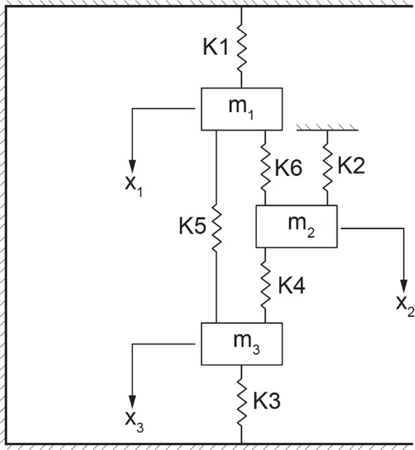
This system has three degrees of freedom  associated with three masses
  . For three masses,
  , and each can move vertically; hence, the number of constraints is
  for each mass. This gives
  . The Lagrangian method is used to find the equations of motion, or three coupled second-order differential equations. We start by writing the kinetic and potential energy expressions of the system and forming the corresponding Lagrangian. The kinetic energy of the system is
  ). For the potential energy, we should use the difference in displacements associated with each spring because the neutral position of the unstressed springs do not contribute to the potential energy. For example, for the spring
  , connecting masses
  and
and  , we should use
  as the variable, or
  . Therefore, the potential energy of the system consisting of the sum of all springs is
  . Note that for this system the kinetic energy is a function of only
  and potential energy a function of
  . Applying Euler-Lagrange equation to each mass, or degree of freedom, we get a system of ODEs, written in matrix form,

For example, the Euler-Lagrange equation associated with mass reads  . But we have
  and
and  . Having information about initial and boundary conditions for displacements and/or velocities, we can obtain the solution of the system’s equations using 20-sim. An initial velocity of 0.2
  is applied to mass
  , for example. The script code is as follows:
parameters
real m1 = 15.0 {kg};
real m2 = 30.0 {kg};
real m3 = 15.0 {kg};
real k1 = 50.0 {N/m};
real k2 = 100.0 {N/m};
real k3 = 50.0 {N/m};
real k4 = 20.0 {N/m};
real k5 = 70.0 {N/m};
real k6 = 10.0 {N/m};
variables
real x1 {m};
real x2 {m};
real x3 {m};
real x1_dot {m/s}; // velocity
real x2_dot {m/s}; // velocity
real x3_dot {m/s}; // velocity
real x1_dot_dot {m/s2}; //acceleration
real x2_dot_dot {m/s2}; //acceleration
real x3_dot_dot {m/s2}; //acceleration
real Fk1 {N}; // force spring k1
real Fk2 {N}; // force spring k2
real Fk3 {N}; // force spring k3
equations
x1_dot_dot = -(1/m1)*((k1+k5+k6)*x1-k6*x2-k5*x3);
x2_dot_dot = -(1/m2)*((k2+k4+k6)*x2-k6*x1-k4*x3);
x3_dot_dot = -(1/m3)*((k3+k4+k5)*x3-k4*x2-k5*x1);
x1_dot = int (x1_dot_dot , 0);
x2_dot = int (x2_dot_dot , 0.2); //initial velocity 0.2m/s
x3_dot = int (x3_dot_dot , 0);
x1 = int (x1_dot , 0.2); //initial displacement 0.2m
x2 = int (x2_dot , 0);
x3 = int (x3_dot , -0.1); //initial displacement -0.1m
Fk1 = k1*x1;
Fk2 = k2*x2;
Fk3 = k3*x3;
The results for displacements of the masses and velocities are shown below, see Figure 2-6.
Here is a video showing how to build and run the model for this example in 20-sim:
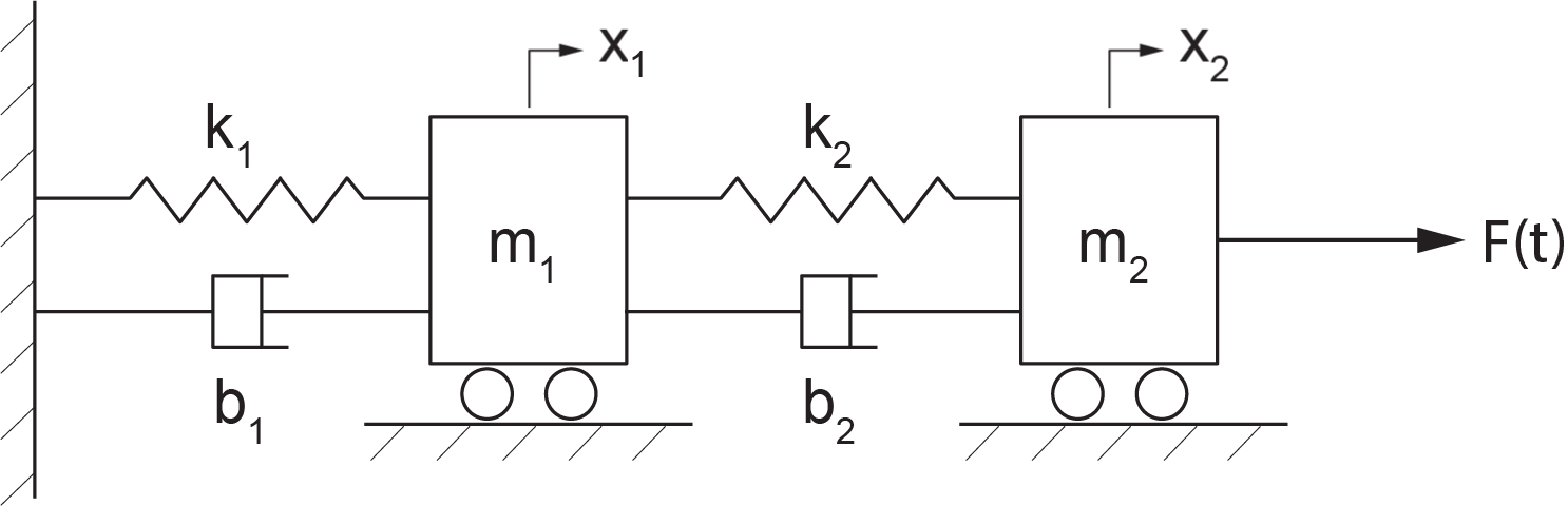
2.12 Example: A System with Energy Dissipation and Applied External Force
We consider a system with two degrees of freedom, as shown in Figure 2-7. The damping coefficients  and
and  and spring stiffness
  and
and  are used to calculate the potential and damping functions and
  , respectively.
The non-conservative Rayleigh energy dissipation function is,  . The derivative of this function with respect to
  gives the damping forces associated with mass
  . The kinetic energy is
  , and potential energy reads
Lagrange’s equation for motion of mass reads  and for mass is
  . Performing the derivatives, we get
Using Lagrange’s equation, with , we get the equations of motion of the system in matrix form as

We use 20-sim to solve the systems equations. A step function is used for applied force. The script code is as follows:
parameters
real m1 = 2.0 {kg};
real m2 = 1.0 {kg};
real k1 = 20.0 {N/m};
real k2 = 30.0 {N/m};
real b1 = 0.1 {N.s/m};
real b2 = 0.05 {N.s/m};
real start_time = 3 {s};
real amplitude = 5 {N};
variables
real x1 {m};
real x2 {m};
real x1_dot {m/s};
real x2_dot {m/s};
real x1_dot_dot {m/s2};
real x2_dot_dot {m/s2};
real F_applied {N}; // applied force
equations
x1_dot_dot = -(b1+b2)/m1*x1_dot+b2/m1*x2_dot-(k1+k2)/m1*x1+k2/m1*x2;
x2_dot_dot = -(1/m2)*(-b2*x1_dot+b2*x2_dot-k2*x1+k2*x2)+F_applied;
x1_dot = int (x1_dot_dot , 0);
x2_dot = int (x2_dot_dot , 0);
x1 = int (x1_dot , 0);
x2 = int (x2_dot , 0);
F_applied = amplitude*step (start_time);
The results for displacements of the masses and applied force are shown below, see Figure 2-8.
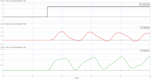
Figure 2-8 Sample results as output from 20-sim
Here is a video showing how to build and run the model for this example in 20-sim:
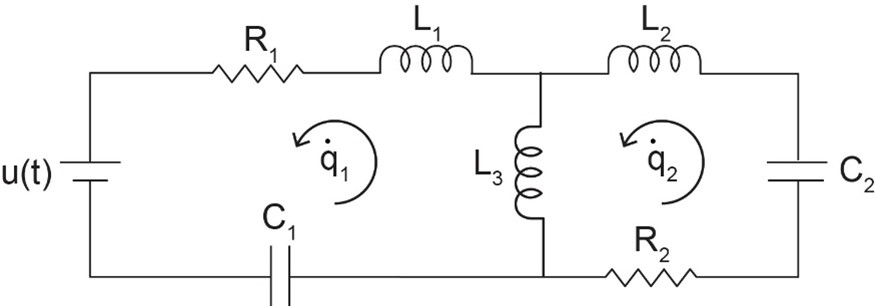
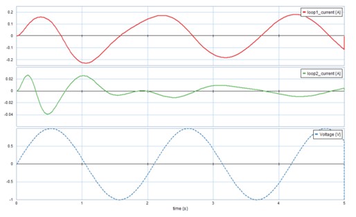
2.13 Example: A Two-Loop Electrical Circuit
For this example, we consider an electrical circuit with two loops/branches. For the system, we have; electric charges and ; resistors  and
and  ; inductors
  ,
,  , and
, and  ; and capacitors
  and
and  as Figure 2-9 shows. The voltage source is
  , connected to loop 1.
For comparison with a typical mechanical system, the equivalent of mass is an inductor; for spring, a capacitor; and for damper, a resistor. Therefore, using the Lagrangian method, we can write the kinetic energy of the system as  . Note that electric charge is analogous to mechanical displacement and electric current to velocity, or
  and
and  . Therefore, e.g., the term
  represents the stored kinetic energy in the corresponding inductor. Similarly, the potential energy is
  . Note that the capacitance is the inverse of stiffness, or
  . The energy dissipation function for the system is
  . Using Langrange’s equation,
  , gives the electric circuit system equations as

One can use rate of charge or the electric current, I as the variable by replacing  in the system’s equations. This gives
  and
and  where
where  and
and  are the voltage across the capacitors, respectively.
We use 20-sim to solve the system equations. The script code is as follow
parameters
real L1 = 0.15 {H};
real L2 = 0.2 {H};
real L3 = 0.25 {H};
real C1 = 0.05 {F};
real C2 = 0.02 {F};
real R1 = 1 {ohm};
real R2 = 2 {ohm};
real omega = 3 {rad/s};
real amplitude = 1;
variables
real q1 {C};
real q2 {C};
real q1_dot {A};
real q2_dot {A};
real q1_dot_dot ;
real q2_dot_dot ;
real Voltage {V}; // applied voltage
equations // equations are manipulated
q2_dot_dot*(L1*L2+L2*L3+L1*L3)=-L3*R1*q1_dot-(L1+L3)*R2*q2_dot-L3/C1*q1-(L1+L3)/C2*q2+Voltage*L3;
q1_dot_dot*(L3) = (L2+L3)*q2_dot_dot+R2*q2_dot+(1/C2)*q2;
q1_dot = int (q1_dot_dot , 0);
q2_dot = int (q2_dot_dot , 0);
q1 = int (q1_dot , 0);
q2 = int (q2_dot , 0);
Voltage = amplitude*sin (omega*time);
Typical plots for current in each loop is shown in Figure 2-10 for a sinusoidal voltage.
2.14 Example: A Compound Atwood’s Machine
Atwood’s machine is a collection of pulleys and masses. This example examines and models the dynamical behavior of this machine as shown in Figure 2-11.
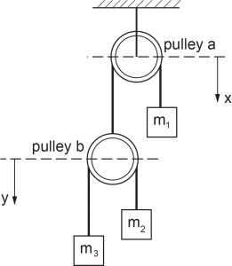
This system has two degrees of freedom  describing the motion of mass and pulley b. Therefore, two ODEs describe the system dynamical behaviour. The massless un-stretchable string length hanging over pulley
  is
is  , and that of pulley
  is
is  . We measure the potential energy with reference to the top of pulley with vertical displacement designated with and similarly from top of pulley with , as shown in Figure 2-11. The kinetic energy reads
  , where , using the geometrical constraints and string lengths,
  . Therefore,
  . Substituting in kinetic energy relation, gives
 ![T= \dfrac{1}{2} [m_1 \dot x^2 + m_2 (\dot y - \dot x)^2 + m_3 (\dot y + \dot x)^2 ]](https://pressbooks.bccampus.ca/engineeringsystems/wp-content/ql-cache/quicklatex.com-216a57e4ace1327fadedc034a824a2a4_l3.png "Rendered by QuickLaTeX.com") . The potential energy reads
. The potential energy reads  . After substituting for
  , and
, and  and algebraic simplifications we get
  , where constant C is given by
  . The Langrange equations in terms of and are
  and
and
 , having
![\begin{equation*} L = T - V = \dfrac{1}{2} [m_1 \dot x^2 + m_2 ( \dot y - \dot x)^2 + m_3 (\dot y + \dot x)^2 ] -xg(m_2 + m_3 - m_1) - yg(m_3 - m_2) \end{equation*}](https://pressbooks.bccampus.ca/engineeringsystems/wp-content/ql-cache/quicklatex.com-449471c56fa7d517d84766ad62960799_l3.png "Rendered by QuickLaTeX.com")
We dropped  , since its differentiation is zero. Hence,


Substituting into the corresponding Lagrange equations, we get the system’s equations of motion as

To simplify the equations, eliminate  by multiplying the first equation by
  and the second one by
  . After some manipulations, we get

We use 20-sim to solve these system equations. The script code is as follows:
parameters
real m1 = 1.0 {kg};
real m2 = 2.0 {kg};
real m3 = 4.0 {kg};
real g = 9.81 {m/s2};
variables
real x {m};
real y {m};
real x_dot {m/s};
real y_dot {m/s};
real x_dot_dot {m/s2};
real y_dot_dot {m/s2};
equations
/* x_dot_dot = (1/(m1+m2+m3))*(-y_dot_dot*(m3-m2)+g*(m1-m2-m3)); */
x_dot_dot = g*(m1-m2-m3)*(m2-m3)/(m1*m2+m1*m3+4*m2*m3);
y_dot_dot = (1/(m3+m2))*((x_dot_dot+g)*(m2-m3));
x_dot = int (x_dot_dot , 0);
y_dot = int (y_dot_dot , 0);
x = int (x_dot , 0);
y = int (y_dot , 0.1);
2.15 Example: Atwood’s Machine with Massive String and Pulley
In the analysis of Atwood’s machine, the pulley and string are usually considered massless. In this example, we include these parts, assuming the string having mass  , total length
  , and linear mass density
  and the pulley with mass
  , radius
  , and moment of inertia
  [19].
[19].
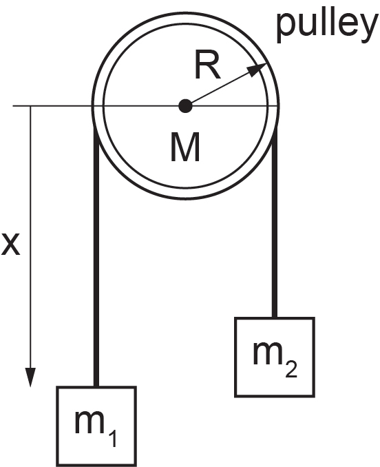
2Datum for potential energy is a horizontal plane at the level of the pulley’s centre. From the datum, the length of hanging string on the two sides of pulley is  . The potential energy is due to the masses and the string mass, or
  . Note that x is measured downward from the datum toward mass . The kinetic energy is due to the masses, string, and the pulley’s angular kinetic energy,
  with angular velocity
  . Therefore,
  . The Lagrangian is written as

The Lagrange is equation reads , or  , after substituting
  . The result reduces to the familiar result of
  for massless string and pulley
  .
.
We use 20-sim to solve these system equations. The script code is as follows:
parameters
real Ms = 2.5 {kg}; // string mass
real L = 2.0 {m}; //string length
real M = 3.0 {kg}; //mass of the pulley
real R = 30.0 {cm}; //radius of the pulley
real g = 9.81 {m/s2}; // grav. acceleration
real m1 = 4.0 {kg};
real m2 = 1.5 {kg};
variables
real x {m}; //vertical displacement
real I {kg.m2}; // pulley moment of inertia
real x_dot {m/s}; // vertical velocity
real x_dot_dot {m/s2}; // vertical acceleration
equations
I = 0.5*M*R^2;
x_dot_dot = g*(m1-m2+(Ms/L)*(x-L))/((m1+m2+(Ms/L)*(L+ pi*R)+I/R^2));
x_dot = int (x_dot_dot , 0.0);
x = int (x_dot , 0);
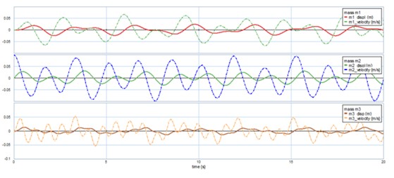
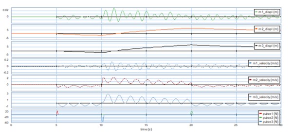
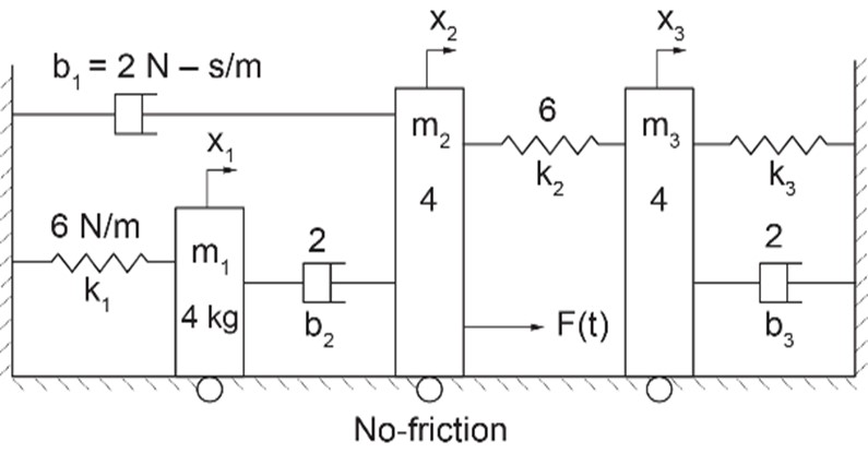
2.16 Example: A Complex Vibrating Mechanical System
For this example, we consider a mechanical system with three degrees of freedom,  , associated with three masses,
 . The arrangement of springs and dampers is shown, with their coefficients, in Figure 2-13, with corresponding stiffness
  and damping
  coefficients. An applied force,
  acting on mass and all wall contact surfaces are considered to have negligible friction.
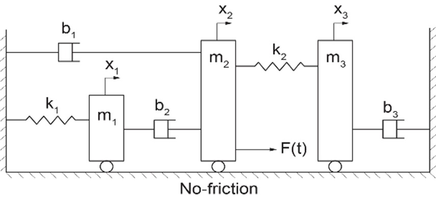
The kinetic energy of the systems reads  and the potential energy is
  . Similarly, the damping function reads
  . The Lagrange’s equations are
  , with
because the applied force is exerted on mass . Performing the differentiations, we can write the equations of the system, as

and  . In matrix form, the system’s equations are

We use 20-sim to solve these system equations. The applied force is composed of three impulses applied at 5, 10, and 20 second. The script code is as follows:
parameters
real m1 = 1.0 {kg};
real m2 = 3.0 {kg};
real m3 = 2.0 {kg};
real k1 = 50.0 {N/m};
real k2 = 30.0 {N/m};
real b1 = 0.1 {N.s/m};
real b2 = 0.2 {N.s/m};
real b3 = 0.3 {N.s/m};
variables
real x1 {m};
real x2 {m};
real x3 {m};
real x1_dot {m/s};
real x2_dot {m/s};
real x3_dot {m/s};
real x1_dot_dot {m/s2};
real x2_dot_dot {m/s2};
real x3_dot_dot {m/s2};
real F_applied1 {N};
real F_applied2 {N};
real F_applied3 {N};
equations
x1_dot_dot = -b2/m1*x1_dot+b2/m1*x2_dot-k1/m1*x1;
x2_dot_dot = -(1/m2)*(-b2*x1_dot+(b1+b2)*x2_dot+k2*x2-k2*x3+F_applied1+F_applied2+F_applied3);
x3_dot_dot = -(1/m3)*(b3*x3_dot-k2*x2+k2*x3);
x1_dot = int (x1_dot_dot , 0);
x2_dot = int (x2_dot_dot , 0);
x3_dot = int (x3_dot_dot , 0);
x1 = int (x1_dot , 0);
x2 = int (x2_dot , 0);
x3 = int (x3_dot , 0);
F_applied1 = 3*impulse (5,0.1);
F_applied2 = 5*impulse (20,0.2);
F_applied3 = -10*impulse (10,0.2);
Sample results are shown in Figure 2-14.
Here is a video showing how to build and run the model for this example in 20-sim:
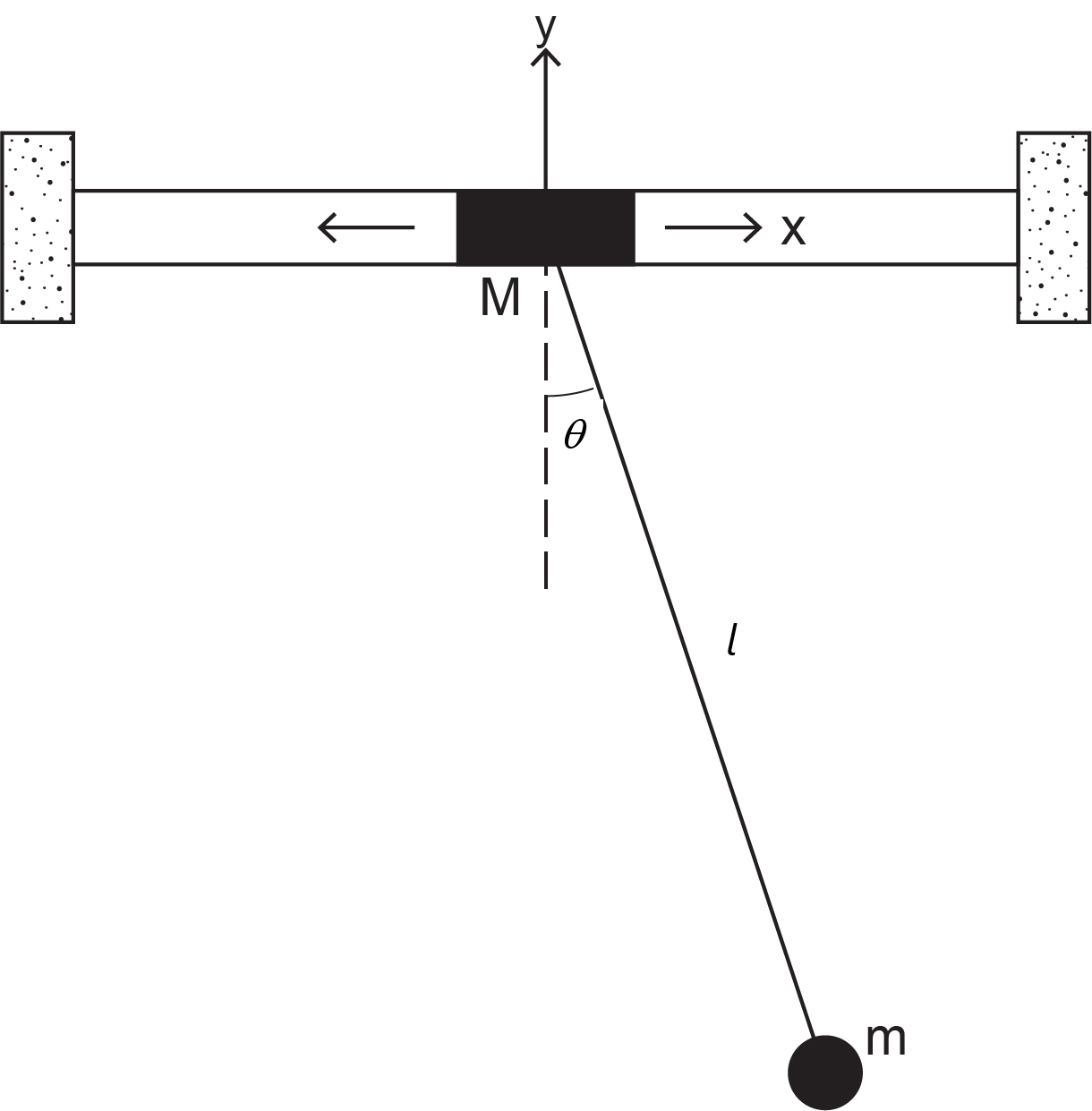
2.17 Example: A Pendulum with Moving Pivot
A simple pendulum with mass hanging from a free-moving pivot with mass . The system has two degrees of freedom: oscillation of pivot,  and pendulum motion about vertical designated by angle
  . The pendulum string with length is massless and unstretchable. We consider the datum at the pivot level and gravitational acceleration
  pointing downwards, as in Figure 2-15.
Mass coordinates read  ; hence, the velocity components are
  . We can write kinetic energy of the system as
![\begin{equation*} T = \frac{m}{2} \left[ (\dot x + l \dot \theta \text{cos} \theta)^2 + (l \dot \theta \text{sin} \theta )^2 \right] + \frac{M}{2} \dot x^2 = \frac{m}{2} (\dot x^2 + l^2 \dot \theta ^2 + 2l \dot x \dot \theta \text{cos} \theta) + \frac{M}{2} \dot x^2 \end{equation*}](https://pressbooks.bccampus.ca/engineeringsystems/wp-content/ql-cache/quicklatex.com-053b4889ad915ab79ccebe63018db523_l3.png "Rendered by QuickLaTeX.com")
Similarly, the potential energy of the systems reads  . Note that the pivot motion is horizontal with coordinates (x, 0). The Lagrange equation for rotational motion with respect to coordinate reads
  , or
, or  . After simplification, we get
  . Note that for fixed pivot (or
  ) we get the familiar result for a simple pendulum. The Lagrange equation for translational motion with respect to coordinate reads
  , or
, or  . After performing differentiation, we get
  . Collectively, the system’s equations of motion are

We use 20-sim to solve these system equations. An initial velocity of 0.5 rad/s is applied to the pendulum. The script code is as follows:
parameters
real m = 0.5 {kg}; // pendulum/bob mass
real M = 1.0 {kg}; // pivot mass
real g = 9.81 {m/s2}; //gravity
real L = 30 {cm}; //pendulum length
variables
real x {m};
real x_dot {m/s};
real x_dot_dot {m/s2};
real theta {rad};
real theta_dot {rad/s};
real theta_dot_dot {rad/s2};
equations
x_dot_dot = (1/cos (theta))*((g/L)*sin (theta)-theta_dot_dot);
theta_dot_dot = (1/(m*L*cos (theta)^2-M-m))*(m*L*sin (theta)*cos (theta)*theta_dot^2-g/L*(m+M)*sin (theta));
x_dot = int (x_dot_dot , 0);
x = int (x_dot , 0);
theta_dot = int (theta_dot_dot , 0.5);
theta = int (theta_dot , 0);
Sample results are shown in Figure 2-16.
Here is a video showing how to build and run the model for this example in 20-sim:
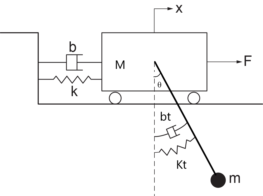
2.18 Example: A Pendulum Attached to a Moving Mass-Spring-Damper System
In this example we consider a system consisting of a pendulum with its pivot attached to the centre of a freely moving mass . The mass is connected to a spring with stiffness  and a damper with damping coefficient . The pendulum bob has a mass of and is attached to a torsional damper with damping coefficient
  and a torsional spring with stiffness
  . The pendulum string is massless and has a length of . We consider the datum at the pivot level and gravitational acceleration pointing downwards, as in Figure 2-17. The system has two degrees of freedom; oscillation of pivot,
  and pendulum motion about vertical direction designated by angle .
The coordinates of mass read  , and its velocity components are
  . We can write kinetic energy of the system as
![\begin{equation*} T = \frac{m}{2} \left[ (\dot x + l \dot \theta \text{cos} \theta )^2 + (l \dot \theta \text{sin} \theta )^2 \right] + \frac{M}{2} \dot x^2 = \frac{m}{2} (\dot x^2 + l^2 \dot \theta ^2 + 2l \dot x \dot \theta \text{cos} \theta ) + \frac{M}{2} \dot x^2 \end{equation*}](https://pressbooks.bccampus.ca/engineeringsystems/wp-content/ql-cache/quicklatex.com-c237beb14cfebcfef8505ccf7129207a_l3.png "Rendered by QuickLaTeX.com")
Similarly, the potential energy of the system reads  . The damping function of the system is
  .
.
The Lagrange equation for rotational motion with respect to coordinate reads  , or
, or  . After simplification, we get
  . The Lagrange equation for translational motion with respect to coordinate reads
  , or
, or  . After performing differentiation, we get
  . Collectively, the system’s equations of motion are

We use 20-sim to solve these system equations. The script code is as follows:
parameters
real m = 0.5 {kg}; // pendulum/bob mass
real M = 1.0 {kg}; // pivot mass
real g = 9.81 {m/s2}; //gravity
real L = 30 {cm}; //pendulum length
real k = 2 {N/m}; // spring stiffness
real kt = 0.5 {N.m/rad}; // torsional stiffness
real bt = 0.5 {N.m.s/rad}; // torsional damping
real b = 0.2 {N.s/m}; // damping
real amplitude = 1; // amplitude of applied force
real omega = 0.5 {rad/s}; // frequency of applied force
variables
real x {m};
real x_dot {m/s};
real x_dot_dot {m/s2};
real theta {rad};
real theta_dot {rad/s};
real theta_dot_dot {rad/s2};
real F_applied {N};
real F_spring {N}; // linear spring force
real T_spring {N.m}; // torsional spring torque
real y; // aux. variable, to help the solver
equations
x = int (x_dot , 0);
x_dot = int (x_dot_dot , 0);
theta = int (theta_dot , 0);
theta_dot = int (theta_dot_dot , 0);
y = -m*L*cos (theta)*(theta_dot_dot);
x_dot_dot = (1/(m+M))*(m*L*sin (theta)*theta_dot^2 + y -k*x-b*x_dot+F_applied);
theta_dot_dot = -g/L*sin (theta) -1/L*cos (theta)*x_dot_dot -1/(m*L^2)*(bt*theta_dot+kt*theta);
F_applied = amplitude*sin (omega*time);
F_spring = k*x;
T_spring = kt*theta;
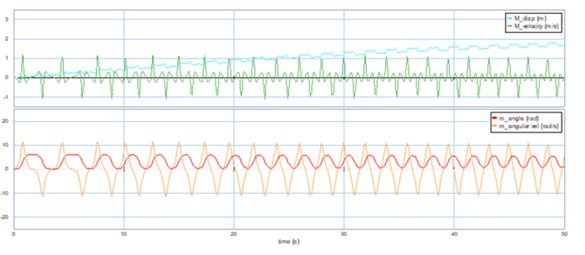
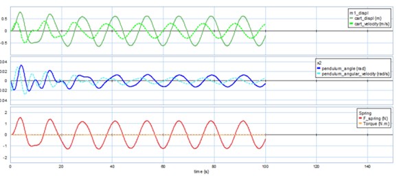
Cart displacement, pendulum angle, and force and torque of the springs are shown in Figure 2-18.
Here is a video showing how to build and run the model for this example in 20-sim:
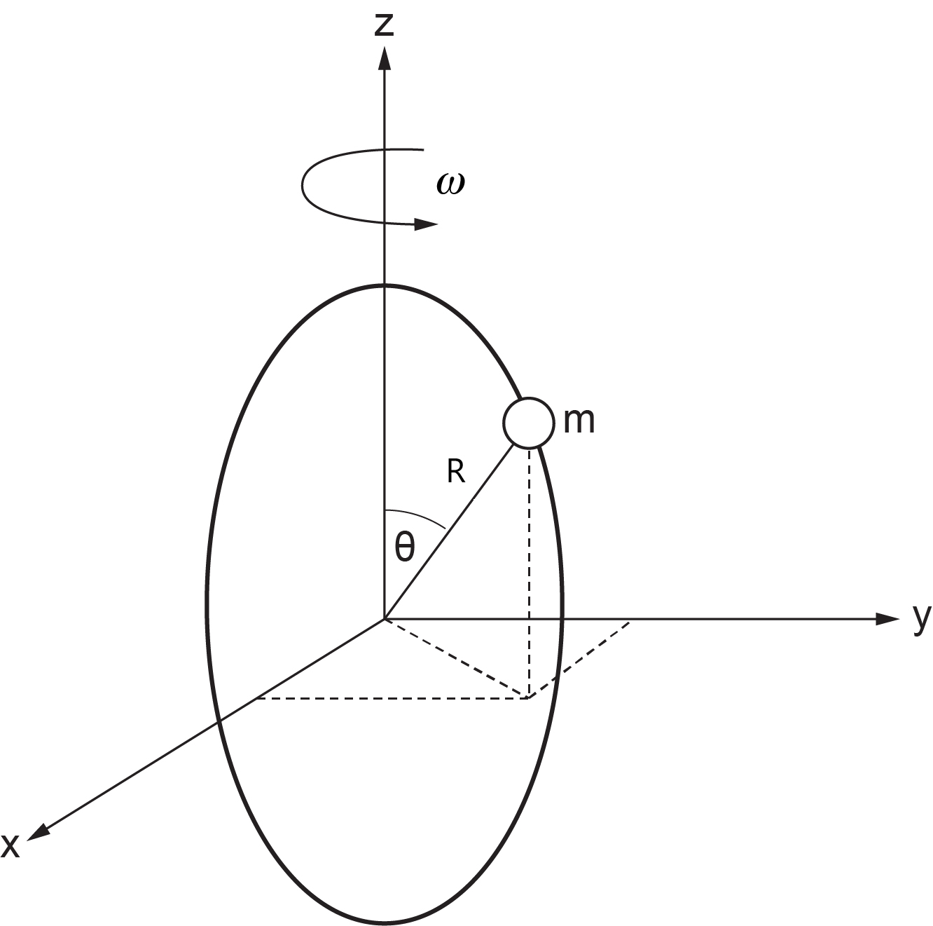
2.19 Example: A Mass Particle Sliding on a Rotating Circular Ring
Figure 2-19 shows a particle with mass sliding on a circular ring with radius . The ring itself is rotating about the -axis with a constant angular velocity  . We want to find the equation of motion for the mass particle.
The generalized coordinate is , the polar angle. We can write the coordinates of the mass particle as  ,
,  , and
, and  . Therefore,
  ,
,  , and
, and  . Therefore, the kinetic energy reads
  ) and after substitution of velocities and simplifications we get
  . Similarly, the potential energy of the mass particle reads
  . Note that the kinetic energy of the particle consists of those resulted from angular velocity
  , defined in spherical coordinates in the
  plane due to sliding of the mass on the circular ring, and the rotational velocity
  , defined in a
  plane parallel to the
  plane at any given time during the motion.
Now we can write the Lagrange’s equations, using Equation (2.12), with the assumption that no friction and non-conservative forces exist, or  . Hence
  . But
. But  ,
,  and
and  . After substitution and rearranging the terms, we get the equation of motion for the mass particle as

We use 20-sim to solve these system equations. An initial angular velocity of 0.2 rad/s is applied to the mass. The script code is as follows:
parameters
real g = 9.81 {m/s2}; //grav. acc.
real R = 40 {cm}; //ring radius
real omega = 0.8 {rad/s}; // ring angular velocity
variables
real theta {rad};
real theta_dot {rad/s};
real theta_dot_dot {rad/s2};
equations
theta_dot_dot= ((1/2)*omega^2*sin (2*theta)+g*sin (theta)/R);
theta_dot = int (theta_dot_dot , 0.0);
theta = int (theta_dot , 0.2);
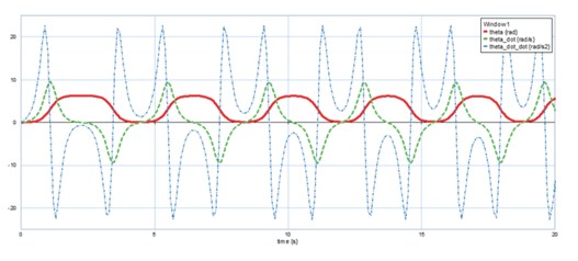
The angular displacement, velocity and acceleration are shown in Figure 2-20.
Here is a video showing how to build and run the model for this example in 20-sim:
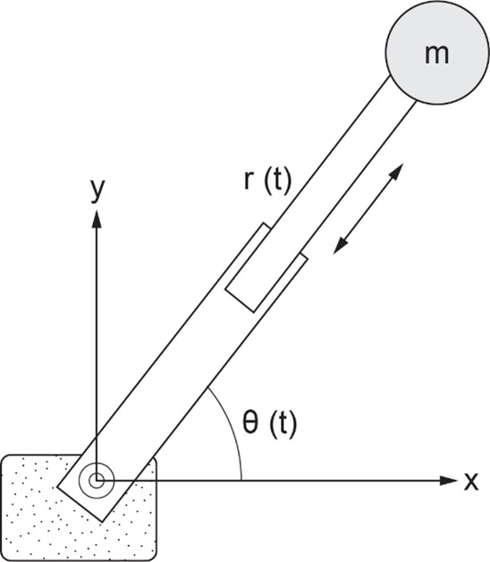
2.20 Example: An Extensible Robotic Arm Rotating in a Plane
Figure 2-21 shows a load with mass is carried by a robotic arm in the plane. The length  of the arm and its angle with respect to -axis are functions of time
  , or
, or  and . The damping coefficients for radial and tangential motions are
  and , respectively.
The generalized coordinates (or degrees of freedom) are  , and corresponding velocities are
  , for mass . We can write the kinetic energy as
  , due to radial and tangential velocities, respectively. The potential energy, with reference to the support, is
  . The damping function is
  . The conservative gravity force due to the load mass is accounted for through the potential function . The force
  and torque
  exerted by the robot-arm motor to move the mass are components of generalized force vector, or
  . Now, we have
  ,
,  ,
,  ,
,  ,
,  ,
,  ,
,  and
and  . Using Equation (2.12), we can write the equations of the motion for the mass , as

We use 20-sim to solve the system equations. The script code is as follows:
parameters
real m = 0.5 {kg}; // load mass
real g = 9.81 {m/s2}; //grav. acc.
real bt = 0.5 {N.m.s/rad}; // tangential damping
real br = 0.2 {N.s/m}; // radial damping
variables
real arm {m};
real arm_dot {m/s};
real arm_dot_dot {m/s2};
real theta {rad};
real theta_dot {rad/s};
real theta_dot_dot {rad/s2};
real F {N}; //applied force
real T {N.m}; // applied torque
equations
arm_dot_dot = (arm*theta_dot^2-g*sin (theta)-br*arm_dot/m+F/m);
theta_dot_dot = (1/(m*arm^2))*(-2*m*arm*arm_dot*theta_dot-m*g*arm*cos (theta)-bt*theta_dot+T);
arm_dot = int (arm_dot_dot , 0);
arm = int (arm_dot , 0.2);
theta_dot = int (theta_dot_dot , 0);
theta = int (theta_dot , 0);
F = sin (0.2*time);
T = 0.2;
Exercise Problems for Chapter 2
Exercises
- Derive Lagrange equation for the system given in example 2.13. Using the Equation Model tool in 20-sim, build a model for this example. Using the numerical data for the parameters, run simulation and analyze the results.
- Derive Lagrange equation for the system given in example 2.14. Using the Equation Model tool in 20-sim, build a model for this example. Using the numerical data for the parameters, run simulation and analyze the results.
- Derive Lagrange equation for the system given in example 2.15. Using the Equation Model tool in 20-sim, build a model for this example. Using the numerical data for the parameters, run simulation and analyze the results.
- Derive Lagrange equation for the system given in example 2.18. Using the Equation Model tool in 20-sim, build a model for this example. Using the numerical data for the parameters, run simulation and analyze the results.
- Derive Lagrange equation for the system given in example 2.20. Using the Equation Model tool in 20-sim, build a model for this example. Using the numerical data for the parameters, run simulation and analyze the results.
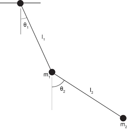
- Using Lagrangian method, derive the system equations for the double pendulum system shown below. Solve the resulting system of ODE’s and draw the angular displacements and velocities
 and
and  ) of mass and for an initial condition of at
  . Also draw the phase diagram (i.e.,
  vs. ) for each mass. Assume that the strings are massless and inextensible.
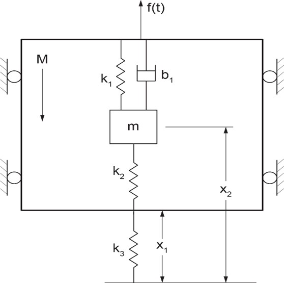
- For the mechanical system given, e.g., an elevator with a mass-spring-damper subsystem, verify the system equations, using Lagrangian method and solve them with 20-sim. The container could be an elevator, e.g., with a mass and is supported by a spring
 and moving vertically, guided by frictionless rollers under load . The subsystem is composed of a mass m, two springs and , and a damper , as shown in the figure below. The gravitational acceleration vector is directed downward,
  .
.

- Repeat the sliding mass on a rotating circular ring example given in section 2.19 assuming
 . Modify the model provided for this example accordingly and run the simulation.
 - Repeat the example given in section 2.16 after adding a mechanical spring
 between mass and the wall. Modify the model provided for this example accordingly and run the simulation.
- Repeat the example given in section 2.17 after replacing the pendulum with a double pendulum. Modify the model provided for this example accordingly and run the simulation.

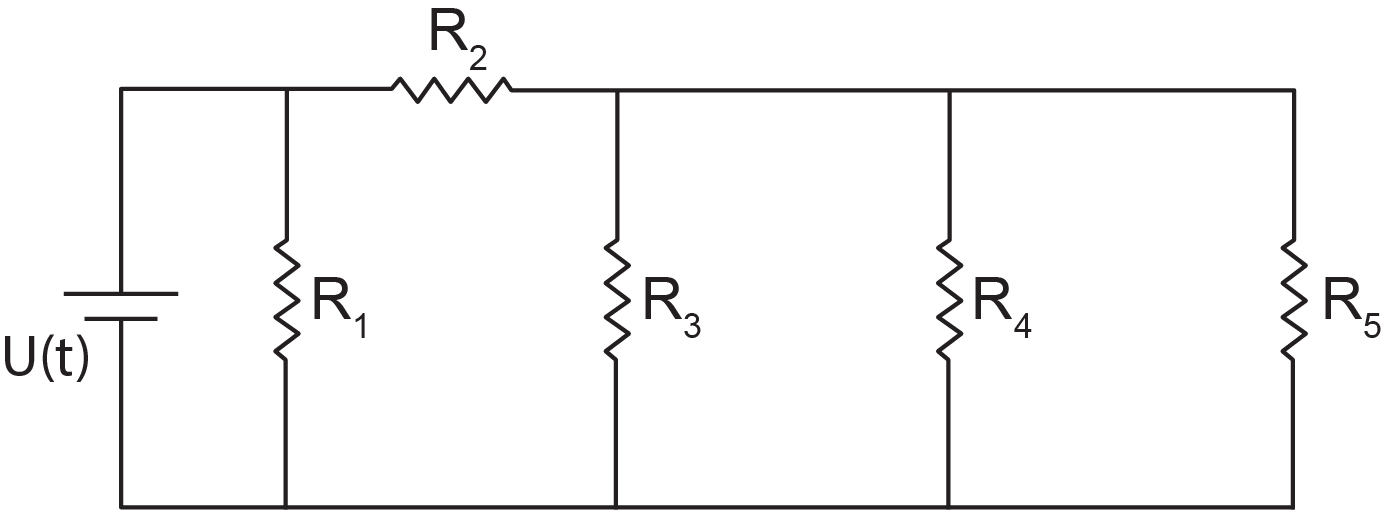
- Derive the system equations for the electrical circuit shown in the below sketch. Use Lagrangian method and solve the resulting system of ODEs with 20-sim.
Media Attributions
- Joseph Louis Lagrange © Zephirin Belliard is licensed under a CC BY (Attribution) license
- William Rowan Hamilton adapted by Quikbik is licensed under a Public Domain license
- Jean le Rond d’Alembert is licensed under a Public Domain license
- Figure2-8_new01
- fig 2-11_edit
