11 Miscellaneous Topics
11.1 Overview
This chapter discusses several topics pertinent to modelling and simulation of systems dynamics with focus on BG method. The reader can consult with these sections as independent topics or as supplementary to previously discussed topics.
11.2 Energy and Power Conjugate Variables
The product of conjugate variables related to a physical quantity should, by definition, give the corresponding quantity. In chapter 3, sections 3.2 and 3.5, we discussed the power variables (effort  and flow
  ) and their relations to the state variables (momentum
  and displacement
  ). The product (
 ) is power—so-called power variables—and integrating them, with respect to time, gives and , respectively. Hence the and are called energy variables. However, further attention to the dimension of the product of the variables, i.e., (
 ), indicates that the dimension of this quantity is not equivalent to that of energy. For example, in the SI system of units, we get
 ![[p.q] = [N.s.m] = [J.s]](https://pressbooks.bccampus.ca/engineeringsystems/wp-content/ql-cache/quicklatex.com-28113a3d6063e40d39bf86db53e483ce_l3.png "Rendered by QuickLaTeX.com") . Therefore, we can call and conjugate power variables because the product () is power. But this definition does not apply to the product (). Instead, the product (
. Therefore, we can call and conjugate power variables because the product () is power. But this definition does not apply to the product (). Instead, the product ( ) or product (
 ) can be defined as true conjugate energy variables.
One can ask the question, what is the relationship among these variables? To investigate further and provide a possible answer, we consider the system energy function  . This functional form is legitimate, since we know that the energy stored, in storage elements
  and
and  , is uniquely defined by state variables (see section 3.5). The total differential change of energy is then
  . In principle,
  . But the partial derivative
  can be ignored at equilibrium state of the system, or when and are kept constant and energy is not changing with time[1]. Now, the total differential change of power
  can be written as the time derivative of energy, or
  . But
. But  and
and  , the effort and flow in BG method, respectively. Therefore, we can write
(11.1) 
Equation (11.1) clearly defines the relationship among power variables (effort and flow ) and state variables (momentum and displacement ) with respect to the power ( ) and energy (
 ) of the system. Note that for a system, we can write this equation for each component and sum it up to get the relation for the system.
From Equation (11.1), we can conclude that by dimensional analysis,  has the dimension of flow and
  the dimension of effort, according to BG terminology. We define these quantities as system flow and effort, or (note that the partial derivative definition is explicitly shown here)
(11.2) 
For example, considering a mass, represented by an -element, its kinetic energy can be written as  , but
, but  , the velocity of the mass or the flow associated with the -element. Similarly, considering a mechanical spring with stiffness
  , represented by a -element, its potential energy can be written as
  , but
, but  , the force acting on the spring or the effort associated with the -element. Equation (11.2) applies analogously to mechanical, electrical, hydraulic, or thermal systems. Note that the energy function relates to the Hamiltonian of the system, [13].
11.3 Including Gravity in BG Models
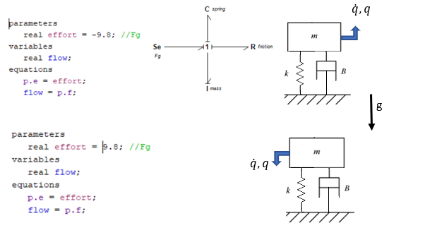
Forces due to gravitational acceleration  can be implemented in a BG model using effort source element
  . But it feeds power to the system when the assigned positive direction of displacement/velocity and the gravitational acceleration vector are in the same direction. Otherwise, the system feeds power into the gravity field, or loses power. In manually drawn BG, the direction of the power bond is drawn from toward the system when the gravity and displacement directions are matched; otherwise, the power bond should be toward the element. In 20-sim, however, it is not possible to draw a power bond pointing toward an element because it is defined as a source element. Hence, a negative value of is assigned to the associated parameter in the corresponding equation model, i.e., −9.81
  (see Figure 11-1). Note that is interpreted as gravitational force per unit mass, here.
11.4 Extracting System Equations from BG Models
Although graphics of BG models can give us some insights into the dynamics of systems before actually solving the systems equations, having the mathematical model consisting of a system of equations is the ultimate goal resulting from a BG model, or for that matter, any model. In the previous sections, we discussed that for a BG model with integral causalities, we can derive a system of ODEs in terms of state variables, i.e., and (see section 3.5). For such a system, the number of equations,  is equal to the sum of number of associated with – elements and number of associated with the – elements. In other words, the system equations are coupled first-order ODEs explicitly given in terms of state variables and can be solved simultaneously using numerical schemes. The solution of these coupled equations is, obviously, easier to obtain for linear systems rather than it is for non-linear systems.
In this section we discuss the procedure and guidelines of how to extract system equations from a BG model. For now, we assume that all storage elements (i.e., – and – elements) in the system are assigned with integral causality strokes. In the next section, we discuss cases when derivative causality and/or algebraic-loop situations may exist in a BG model, along with the definitions and resulting consequences for such systems equations.
Referring to the energy management of a system, we have already discussed that the energy input to a system is partially stored in storages and the rest is dissipated through dissipaters. Therefore, the storage elements are key elements for studying the dynamics of any system. This principle also applies to the BG models, and we use it to extract system equations.
The system equations can be given in a general form as  where
where  , the vector representing time derivative of state variables,
  , the vector representing the inputs, with indices
  and
and  . One can expand this functional to get
(11.3) 
After building the BG model for a system, we ask the following two key questions, [21]:
Q1: What does each component/element send to the system?
Q2: What does the system send back to the storage components/elements?
Each question guides us to list the corresponding relations involving the state variables and performing some manipulations to write the system equations in terms of the state variables, using the general guideline of on and on . The following steps can be used to extract the system equations:
- Build the BG model and assign causalities, with preferred integral causalities.
- Simplify the BG model, as far as possible.
- Assign labels as numbers to each power bond in the BG model. The order of numbering is arbitrary.
- Answer Q1, in terms of all efforts or flows input into the system.
- Answer Q2, in terms of all ’s on ’s and all ’s on ’s, or momenta (or their derivatives) associated with the inertia elements and displacements (or their derivatives) associated with the capacity elements.
- Apply constraints implemented by 1- and 0- junction elements and perform algebraic manipulations to write the system equations only in terms of state variables, as independent variables with inputs and components’ properties as parameters.
Now, we present some worked-out examples to demonstrate the application of the above mentioned procedure.
11.4.1 Example: System Equations for a Mechanical System
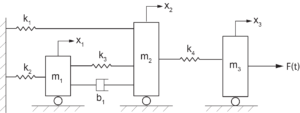
For this example, we consider a mechanical system as shown in Figure 11-2. This systems has three DOF associated with three masses. The number of state variables is seven, associated with the storage elements, three masses, and four springs. The positive displacements are considered as shown, and tension forces are positive (+T).
Solution:
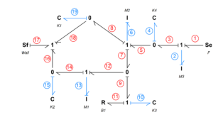
We first build the BG model, either manually or using the tools available through 20-sim, with all power bonds labelled, as shown in Figure 11-3. As mentioned, the labels are arbitrary; they merely help bookkeeping of the variables involved without affecting final solution of the system equations. Therefore, the state variables are:  associated with the momenta of the masses and
  displacements of the mechanical springs. The corresponding power bonds to these elements are colour coded (see Figure 11-3). The system equations are ODEs consisting of these state variables. To extract the system equations, we ask two key questions (see section 11.4) and list their corresponding answers, using the power bond labels and causality assignments in terms of BG symbols and , as follows:
Q1: What does each component/element send to the system?
The inputs to the system are from elements at the boundary of the system associated with bonds 1, 2, 4, 6, 10, 11, 13, 15, 17, and 19, as listed in Table 11-1.
| Power bond label # | System input/relation |
| 1 |  |
| 2 |  |
| 4 |  |
| 6 |  |
| 10 |  |
| 11 |  |
| 13 |  |
| 15 |  |
| 17 |  |
| 19 |  |
Next, we list the relations to answer the second question:
Q2: What does the system send back to the storage components/elements?
Here, we are only interested in storage elements, as shown by colour-coded bonds in Figure 11-3. For example, considering power bond number 2, the system sends an effort signal (or rate of momentum) to the -element representing the mass  . Therefore, we can write
  . Similarly, considering power bond number 15, the system sends a flow signal (or rate of displacement) to the -element representing the spring
  . Therefore, we can write
  . Table 11-2 lists all relations corresponding to storage elements.
| Power bond label #(element) | Storage element/relation | Relations, using constraints |
2 ( ) ) |
 |
 |
4 ( ) ) |
 |
 |
6 ( ) ) |
 |
 |
10 ( ) ) |
 |
 |
13 ( ) ) |
 |
 |
15 ( ) ) |
|
 |
19 ( ) ) |
 |
 |
In the relations listed in the third column of Table 11-2, we used the constraints resulted from 1- and 0-junctions and elements’ constitutive equations, and included the relations from Table 11-1. The final relations are given in bold. Finally, after some manipulations, we can write the system equations in terms of seven state variables in matrix form, as given in Equation (11.4).
(11.4) 
11.4.2 Example: System Equations for an Electrical System
For this example, we consider the electrical system and BG model given in section 7.6 and shown in Figure 7-8. The system has two loops. The number of state variables is three, associated with the storage elements, two inductors and one capacitor.
Solution:
Figure 11-4 shows the BG model with labelled power bonds for this system. The power bonds associated with storage elements, hence state variables, are colour coded.
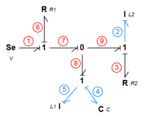
As mentioned, the labels are arbitrary and they merely help bookkeeping of the variables involved without affecting final solution of the system equations. The state variables are:  associated with the momenta of the inductors, and
  , electrical charge of the capacitor. The system equations are ODEs consisting of these variables. To extract the system equations, we ask two key questions (see section 11.4) and list their corresponding answers, using the power bond labels and causality assignments in terms of BG symbols e and f, as follows:
Q1: What does each component/element send to the system?
The inputs to the system are from elements at the boundary of the system associated with bonds
1, 2, 3, 4, 5, and 6, as listed in Table 11-3.
| Power bond label | System input/relation |
| 1 |  |
| 2 |  |
| 3 |  |
| 4 |  |
| 5 |  |
| 6 |  |
Next, we list the relations to answer the second question:
Q2: What does the system send back to the storage components/elements?
Here, we are only interested in storage elements, as shown by colour-coded bonds in Figure 11-4. For example, considering power bond number 2, the system sends an effort signal (or rate of momentum/flux linkage) to the -element representing the inductor  . Therefore, we can write
  . Similarly, considering power bond number 4, the system sends a flow signal (i.e., current or rate of charge) to the -element representing the capacitor
  . Therefore, we can write . Table 11-4 lists all relations corresponding to storage elements.
| Power bond label (element) | Storage element/relation | Relations, using constraints |
2 ( ) ) |
|
 |
4 ( ) ) |
|
 |
5 ( ) ) |
 |
 |
Note that  . In the relations listed in the third column of Table 11-4, we use the constraints resulted from 1- and 0-junctions and elements’ constitutive equations, and included the relations from Table 11-3. The final relations are given in bold. Finally, we can write the system equations, after some manipulations, in terms of three state variables in matrix form, as given in Equation (11.5).
(11.5) 
11.5 Derivative Causality and Algebraic Loop: Implicit System Equations
When assigning causality strokes to a BG model, three scenarios may occur [20], [21]. These scenarios are:
- all causality strokes are possible to be assigned as preferred integral causalities;
- at least one storage element (– or – element) cannot be assigned with integral
causality; instead derivative causality is forced upon the element; or - there is more than one option for having a BG model with assigned integral causalities for the given system, a so-called algebraic loop.
All of these scenarios are legitimate in terms of BG modelling rules, and with red colour-coded causality strokes, 20-sim provides warnings, not errors, for scenarios 2 and 3 as listed above. As mentioned, scenario 1 is desirable and preferred. For this scenario, the system equations can be derived explicitly in terms of state variables as a system of coupled first-order ODEs. The solution of the system of equations provides the answers for the generalized momenta and displacements associated with storage elements. After having the solutions for system equations, we can calculate other desired quantities related to the system.
For the second scenario, the system equations are not independent, i.e., implicit. In other words, the equations related to the storage elements with integral causalities are independent; pertinent state variables can be uniquely calculated by solving these equations, simultaneously. But the equation related to the storage element with derivative causality is not independent; it relates algebraically to the independent equations. Therefore, the related state variable for the element with derivative causality can be calculated using the solution of those of the independent variables. The mathematical dependence of the equation for the derivatively causalled element indicates that the dynamics of the element are related to and defined by the other storage elements in the system. In addition, for the derivative causality case, we may have to force more than one element having non-integral causalities.
For the third scenario, after assigning integral causalities for some of the elements in a definite manner, we face one or more options and have to make choices for one or more elements and arbitrarily assign them with causalities. The resulting system equations are again independent coupled ODEs and can be simultaneously solved to find their solutions. However, during the manipulation, we encounter an implicit equation (or equations) for a particular state variable (or its derivative) which is a function of inputs and itself as well—an algebraic loop. For linear systems/elements, the algebraic-loop situation does not pose a problem; however, for non-linear systems/components, this makes it more difficult to manipulate the equations to find their solutions.
Note that an algebraic loop may occur at several levels and, hence, make it harder to manipulate the equations. This is when, after selecting an assigning causality stroke for an element arbitrarily, further selection(s) should be made to proceed.
For both scenarios, derivative causalities and algebraic loop, the fact that they appear in a BG model is useful information about the system and/or assumptions made for the model, even before solving the resulting equations. In many cases, the modeller can improve the system with additional components, usually of the types of  – element.
As mentioned, 20-sim sends warning messages, but no error messages when derivative causalities and algebraic loop exist. The resulted system equations can be solved by solvers available, and the system simulation and design can proceed as usual.
In further sections, we present some examples to demonstrate the derivative causality and algebraic-loop cases.
11.5.1 Example: BG Model with Derivative Causality
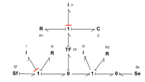
We consider the BG model shown in Figure 11-5. The colour-coded bonds associated with two inertia -elements are forced, having non-integral causalities or derivative causality. This can be vividly explored by starting assigning causality from  -element sending a flow signal to the adjacent 1-junction. Therefore, all other connecting bonds to this 1-junction should have their causality strokes at the ports connecting to this 1-junction. This requirement forces the associated -element to have a derivative causality, or sending effort signal, instead of receiving it for being integrally causalled, to the 1-junction. Similarly, the -element
  is forced to have derivative causality. As a result, the momenta of these two -elements (i.e. and ) will depend on the remaining storage elements, i.e., -element
  and -element , and can be calculated having the corresponding solutions for – and – elements. For further reading, consult with references cited as [5], [20], [21], and [30].
As mentioned, in 20-sim a warning message appears on the screen when derivative causality exists in the BG model. But the software solver tools take care of this and solve the system equations. This capability is useful for practical applications in design of the systems.
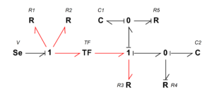
11.5.2 Example: BG Model with Algebraic Loop
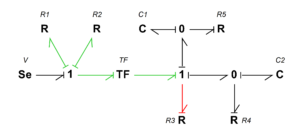
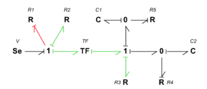
We consider the BG model shown in Figure 11-6. Starting with the process of assigning causalities, we realize that the colour-coded bonds can’t be integrally assigned and present options. In other words, to proceed further with assigning causalities to the whole system’s BG model, we require to make a selection arbitrarily. Usually, the selection can be more easily made with -elements, since it can be assigned with neutral causality. For example, if we select the element  and assign causality stroke to it such that it sends a flow signal to the adjacent 1-junction, then the remaining bonds’ causality strokes can be assigned, as shown colour coded in Figure 11-7. Alternatively, element
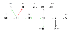
  or
or  could be selected as an option. The corresponding BG models and related assigned causalities are shown in Figure 11-8 and Figure 11-9, respectively.
For further reading, consult with references cited as [5], [20], [21], and [30].
As mentioned, in 20-sim, a warning message appears on the screen when algebraic loop causality exists in the BG model. But the software solver tools take care of this and solve the system equations. This capability is useful for practical applications in design of the systems.
11.6 Thermal Systems: Pseudo Bond Graph
Thermal systems are unique in terms of BG modelling. They are closely analogous to electrical systems. In practice, to analyze thermal systems, we use this analogy to build models as thermal networks, similar to electrical networks, [39], [40].
Considering heat conduction through a solid slab, e.g., the temperature difference  (analogous to voltage) and heat flow rate
  (analogous to electrical current) satisfy
  . The quantity
  (analogous to electrical resistance) is thermal resistance with dimension [K/W], in
  , where,
  is the length across which the applies;
  is the cross-sectional area for heat flow, and
  is the thermal conductivity of the material. Intuitively, this analogy suggests to consider temperature as the effort and the heat flow rate as the flow when building BG models for thermal systems. With this assumption at hand, the product (
 ) would be considered as power variables, or the dimension of this quantity should be as of that for power. However, close examination of the dimension for the product () gives its dimension as
 ![[(T\dot Q_{th})] = K \cdot W](https://pressbooks.bccampus.ca/engineeringsystems/wp-content/ql-cache/quicklatex.com-653b673f38ea3f787dec941dcc3b5cf3_l3.png "Rendered by QuickLaTeX.com") , or
, or  . Therefore, according to BG modelling rules, we cannot accept temperature and heat flow rate as conjugate power variables. This discrepancy leads us to call such a BG model a pseudo bond graph (pseudo BG), for which temperature is the effort and heat flow rate is the flow. This is acceptable as far as the thermal system is the only system involved and the modeller is aware of the fact that the “power” variables are not defined fully and correctly in the related thermal pseudo BG model. However, for multi-domain systems, the exchange of power between a thermal sub-system part and other domains of the system becomes problematic.
The solution to this challenge comes from the second law of thermodynamics, which guides us to consider the flow in the BG model as the entropy rate, instead of heat flow rate. Recall that entropy is a state function, and for a reversible system, we have the relationship  for exchange of heat
  and entropy
  using temperature
  , [41]. Therefore, the heat flow rate is
  . The dimension of
  , the entropy rate, is then [
 ]. Therefore the dimension of the power variables, or (
 ) is [
 ], as it should be; hence, we can accept the temperature as the effort and entropy rate as the flow (or entropy as displacement) in BG model for a thermal system. Table 11-5 shows the variables involved in Pseudo BG and BG models for thermal systems.
| Model | Effort | Flow | Power | System |
|---|---|---|---|---|
| Pseudo BG | temperature | heat flow rate | ill-defined | single thermal domain |
| BG | temperature | entropy rate | defined | multi-domain |

