Frequency Analysis: Bode Plots and Transfer Function

Mehrzad Tabatabaian

10 Frequency Analysis: Bode Plots and Transfer Function

10.1 Overview

Studying the behaviour of systems with respect to time is the primary approach for systems modelling and analysis. However, when a system behaves in a repetitive mode under some applied load and/or boundary conditions—a quasi-static mode—we are interested in the changes in terms of the inherently-involved frequencies of the system rather than the details of instantaneous variations with respect to time. Therefore, transforming the domain of analysis from time to frequency provides us with useful and important information about the behaviour of systems. For example, identifying characteristics of a system—such as its natural frequency, behaviour at large and small frequencies, and magnitude of certain quantities at specific frequencies—provides useful insights in terms of system analysis, design, and control.

In this section, we present a brief background of frequency analysis and methods with focus on Bode plot method and transfer function, with worked-out examples. However, this textbook does not present a full discussion of control theory and related methods for system analysis.

For further reading, consult with references cited in this chapter. 20-sim has tools for performing frequency analysis using BG models and for drawing Bode plots for systems. Through some examples, we will demonstrate how to use these tools.

10.2 Background

Performing analysis in frequency domain requires a transformation from time domain to frequency domain. Having a mathematical model describing the behaviour of a system, we can use a transformer to convert the governing equations from time domain to frequency domain $\omega$ . Using applied engineering mathematics, we usually employ Laplace and/or Fourier transforms for such an operation. The Laplace transform (defined in complex $s$ -domain) is a more general case of Fourier’s transform (defined in $\omega$ -domain), as given below for transforming a function of time $F(t)$ , [12], [35].

(10.1) $\begin{equation*} \begin{dcases} \tilde{F}(s)=\mathcal{L}(F(t))={\int_{0}^{t}}e^{-st}F(t)dt\:\textit{,Laplace}\\ \check{F}(\omega)=\mathcal{F}(F(t))= {\int_{-\infty}^{+\infty}}e^{-j\omega{t}}F(t){dt}\:,\textit{Fourier}\\ \end{dcases} \end{equation*}$

where $j=\sqrt{-1}$ and for $s=j\omega$ these two transforms are comparable. Note that, in principle, $s=\sigma+{j\omega}$ but the real part, $\sigma$ of complex variable $s$ , is not included here since we are interested in equilibrium at a steady state in frequency analysis. Application of these transforms greatly simplifies the solutions of system equations, both for ODEs and PDEs. The original functions in time domain can be calculated back using the inverse transforms of Laplace and Fourier, given as

Jean Baptiste Joseph Fourier (1768–1830)

(10.2) $\begin{equation*} \begin{dcases} \textit{F}(t)=\mathcal{L}^{-1}({\tilde{F}(s))=\dfrac{1}{2\pi{j}}{\int_{-j\omega}^{j\omega}}e^{st}\tilde{F}(s)ds\textit{, inverse Laplace}\\ \textit{F}(t)=\mathcal{F}^{-1}(\check{F}(\omega))=\dfrac{1}{2\pi} {\int_{-\infty}^{+\infty}}e^{j\omega{t}}\check{F}(\omega){d}\omega\:,\textit{inverse Fourier}\\ \end{dcases} \end{equation*}$

In control theory for systems, several methods are used for studying system behaviour and design, including Bode and Nichols plots requiring frequency-domain response representation, root-locus method requiring complex-domain pole-zero representation, and polynomial-domain design requiring transfer-function representation [31], [36]. A transfer function, by definition, is the ratio of the output signal (i.e., magnitude, power) of a system over selected input signal values. Among these methods, we focus on Bode plots for application in system design using BG models. Bode plots are used for linear systems or linearized non-linear systems. For more detail, see Reference Manual 20-sim 4.6. To access the manual, from the 20-sim Editor window, go to Help, and then select Manual (PDF).

10.3 Motivational Example: A Linear System

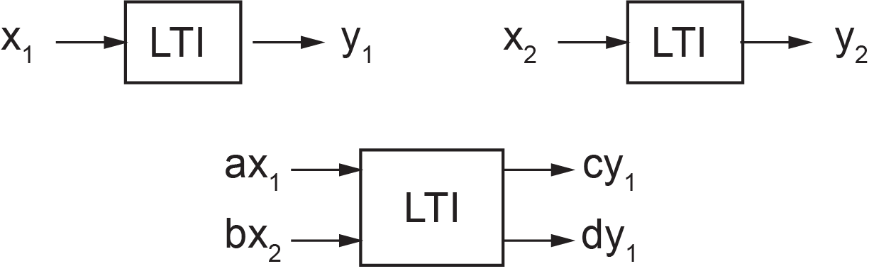
A linear system, or LTI (linear time invariant), is a system for which the linear combination of output of a set of inputs is equal to the sum of outputs resulting from each input, e.g., as shown in Figure 10‑1.

Figure 10-1 Linear system sketch for processing inputs and outputs

Considering a proportional integral (PI) controller (for which the output is equal to the input multiplied by a constant and added to the integral of the input), we provide a sinusoidal signal input with frequency of 0.5 rad/s (or $\dfrac{0.5}{2\pi}Hz$ ) given as 0.5 $t$ . Assuming the constant multiplier to be 2, we get the output as $F(t)=2\sin0.5t+\int\sin0.5t\:{dt}=2(\sin0.5t-\cos0.5t$ ). From the output, we observe that the frequency remains the same as that of the input. Now, by multiplying $\dfrac{\sqrt{2}}{\sqrt{2}}=1$ to the output, we rewrite it as a single sinusoidal function, or:

$F(t)=2\sqrt{2}(\dfrac{1}{\sqrt{2}}\sin0.5t-\dfrac{1}{\sqrt{2}}\cos0.5t)=2\sqrt{2}(\cos\dfrac{\pi}{4}\sin0.5t-\sin\dfrac{\pi}{4}\cos0.5t)=2\sqrt{2}\sin(0.5t-\dfrac{\pi}{4}).$

Therefore, the input amplitude is magnified by a factor of $2\sqrt{2}$ , frequency remains the same as mentioned, and a phase change of $-\dfrac{\pi}{4}=-45^{\circ}$ is introduced to the output signal by the PI controller. But one can ask the question: what would be the controller response to a similar signal with a different frequency? For example, if we repeat the same calculation for an input signal given as $\sin0.8t$ , we get the response $\dfrac{\sqrt{89}}{4}\sin(0.8t-32.01^{\circ})$ . To find the response to a spectrum of input frequencies, in principle we can repeat similar calculations and analyze the system behaviour. Table 10‑1 shows some typical response result for input signals of the form $\sin\omega{t}$ into a PI controller.

Table 10‑1 Response of a PI controller to a sinusoidal signal, $\sin\omega{t}$
Frequency (rad/s), $\omega$	Response Amplitude	Response Phase (deg.)
0.1	10.198	-78.690
0.2	5.385	-68.199
0.3	3.887	-59.036
0.4	3.202	-51.340
0.5	2.828	-45.000
0.6	2.603	-39.806
0.7	2.458	-35.538
0.8	2.358	-32.005
0.9	2.288	-29.055
1	2.236	-26.565
2	2.062	-14.036
3	2.028	-9.462
4	2.016	-7.125
5	2.010	-5.711
6	2.007	-4.764
7	2.005	-4.086
8	2.004	-3.576
9	2.003	-3.180
10	2.002	-2.862

One can make graphs of the response amplitude and phase changes versus input frequency to study the behaviour of the PI controller used in this example.

10.4 Bode Plots and Cutoff Frequency

The results of the calculations mentioned in section 10.3 motivate us to look for a more general and practical method of frequency analysis of systems. The calculations presented are laborious, although new computer tools, e.g., Excel or even computer coding can speed up the process. However, Hendrik Wade Bode, working at Bell Labs in the 1930s, suggested a more practical and now commonly used graphical method—Bode plots, [21], [31], [37], [38]. This method has a wide range of applications in system dynamics, control, and design. An important outcome of having Bode plots for a system is a quick visual insight into the system’s dynamical behaviour for a wide range of frequencies.

In this section, we present the basic idea and some formulas related to Bode plots and what they intend to represent when applied to a system.

Following the example presented in section 10.3, we assume, without losing generality, to have an input sinusoidal signal to the PI controller with frequency $\omega$ given as $A_0\sin\omega{t}$ . The output is, then, $A\sin(\omega{t}+\varphi)$ with amplitude $A$ and phase $\varphi$ . The relations for the output amplitude and phase angle depend on the PI controller specifications. For our example having a proportionality factor of two and an integration, using similar manipulations as those given in section 10.3, we find $A=A_0\sqrt{4+1/\omega^{2}$ and $\varphi=\tan^{-1}(-\dfrac{1}{2\omega})$ . Now, after transforming the input and output signals to the Laplace $s$ -domain, using Laplace transform (see Equation (10.1)), we get $\mathcal{L}\underbrace{(A_0\sin\omega{t})}_{input}=A_0\dfrac{\omega}{s^{2}+\omega^{2}}$ and $\mathcal{L}\underbrace{(2A_0\sin\omega{t}+{\smallint}A_0\sin\omega{t})}_{output}=A_0(\dfrac{2\omega}{s^{2}+\omega^{2}}+\dfrac{\omega/s}{s^{2}+\omega^{2}})$ . The transfer function $G(s)$ (also referred to as gain function) is defined as the ratio of the output amplitude over input amplitude. For our examples, we get, after some simplifications, $G(s)=2+\dfrac{1}{s}$ . Having the transfer function, we can substitute $s=j\omega$ , to transform from $s$ -domain to $\omega$ -domain, guided by Equation (10.1). Therefore, $G(\omega)=G(s)|_{s=j\omega}=2+\dfrac{1}{j\omega}$ , or the transfer function in frequency domain. This is a function of a complex variable and can be written, in general, as its real and imaginary parts or $G(\omega)=\mathfrak{R}+j\mathfrak{J}$ . Therefore, after some manipulations, we get $G(\omega)=2+\dfrac{1}{j\omega}=2-\dfrac{j}{\omega}$ . This gives the real part $\mathfrak{R}=2$ and imaginary part $\mathfrak{J}=-1/\omega$ . Therefore, the magnitude of the transfer function is $|{G}|=\sqrt{4+1/\omega^{2}}$ . The relations for transfer function including its magnitude and phase are summarized in Equation (10.3).

(10.3) $\begin{equation*} \begin{dcases} \textit{G}(\omega)=\mathfrak{R}+j\mathfrak{J}\\ |\textit{G}(\omega)|=\sqrt{\mathfrak{R}^{2}+\mathfrak{J}^{2}}\\ \varphi=\tan^{-1}(\frac{\mathfrak{J}}{\mathfrak{R}})\\ \end{dcases} \end{equation*}$

A set of plots consisting of magnitude $|G(\omega)|$ and $\varphi$ versus logarithm (at base 10) of $\omega$ is called Bode plots. However, magnitude is traditionally measured in decibel (dB), phase angle in degrees, and frequency as logarithm of frequency in rad/s (or in Hz).

Recall that dB (one tenth of a bel) is a unit for measuring the power of a signal with reference to a threshold. For example, the threshold for human hearing is $10^{-12}W/m^{2}$ , given as power intensity; dB is measured in logarithm of the power ratios at base ten, or $dB=10\log_{10}\dfrac{power\:out}{power\:in}$ . But since power of a wave signal is proportional to its amplitude squared, then we get $dB=20\log_{10}\dfrac{amplitude\:out}{amplitude\:in}$ , or

(10.4) $\begin{equation*} \textit{d}B=20\log_{10}|G(\omega)|\\ \end{dcases} \end{equation*}$

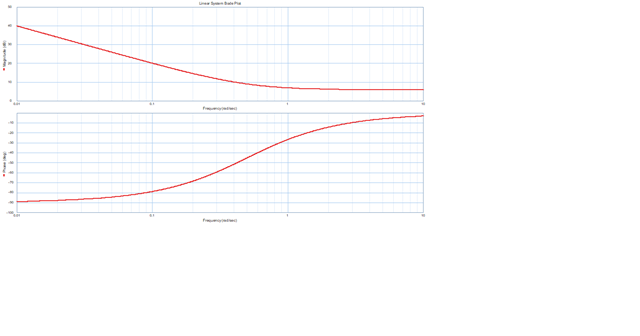
Therefore, Bode plots are composed of two charts: signal gain in dB and phase in degrees versus logarithm of $\omega$ , usually given in a single graph chart. The graphs in Figure 10‑4 show the Bode plots for the PI controller, generated using 20-sim. The tools available for drawing Bode plots in 20-sim can also be used when a transfer function is available or calculated and also after a BG model is built for systems. For this example, we calculated the transfer function and used it to draw the corresponding Bode plots. For drawing the corresponding Bode plots, follow these steps:

From the Editor window, go to Tools, select Frequency Domain Toolbox, and then select Linear System Editor. The 20-sim Linear System Editor window opens, as shown in Figure 10‑2.

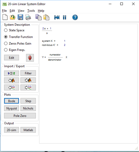
Figure 10‑2 Linear System Editor interface in 20-sim

Select Transfer Function and click on the Edit A window opens in which you can enter the coefficients of the transfer function, as shown in Figure 10‑3.
Enter the desired transfer function as a polynomial fraction with numerator and denominator polynomials with their corresponding coefficients in descending power of $s$ . For this example, having $G(s)=2+\dfrac{1}{s}=\dfrac{2{s}+1}{s},$ the coefficients for the numerator polynomial are (2, 1) and for the denominator polynomial are (1, 0). Note the zero term, i.e., the coefficient for the term $s^{0}$ , or the constant term. A space can be used instead of a comma, to separate the coefficients.
Click on Apply and then OK This takes you back to the Linear System Editor window with the transfer function listed. Double check the resulted transfer function to make sure it is entered correctly into 20-sim.

Figure 10‑3 Transfer Function Editor interface in 20-sim
From the 20-sim System Editor window (see Figure 10‑2) under Plots, select Bode. The Bode Plot window opens with the corresponding Bode plots, as shown in Figure 10‑4. From these plots, we can conclude that the PI controller is a high-pass filter system because it passes through the high frequency signals but attenuates low frequency signals. The gain for low frequency signals decreases linearly with a slope of 20 dB per decade from 40 dB. The phase change is from close to $-90^{\circ}$ at low frequencies to null at high frequencies. Therefore, the PI controller is in phase with the input signals at high frequencies and out of phase, by about $-90^{\circ}$ , at low frequencies.
The asymptotes to the high frequency and low frequency gains intersect at a point defined as the cutoff frequency, $\omega_{b}$ (also referred to as corner or break frequency). This frequency is defined when the output power reaches to 50% of the input signal power (so-called half-power point), or $|dB|=\Big|10\log_{10}\dfrac{power\:out}{power\:in}\Big|=|10\log_{10}0.5|=\Big|20\log_{10}\underbrace{0.5^{0.5}}_{=1/\sqrt{2}}\Big|\cong3$ .
The 3dB-point is the standard method of finding cut off frequency from the Bode plot gain chart. For this example, the asymptote to the high frequency gain (i.e., the horizontal line as the frequency $\rightarrow\infty$ ) is at about 6.02 dB. Hence, the cutoff frequency corresponds to the point at 6.02+3=9.02 dB, or $|G(\omega)|=2.825$ using Equation (10.4). This gives the cutoff frequency of $\omega_{b}=0.5013$ rad/s, using $|G(\omega)|=2.825=\sqrt{4+1/\omega^{2}$ . At the cutoff frequency the phase reads $-45$ deg, using $\varphi=\tan^{-1}(-\dfrac{1}{2\times0.5013})$ , after conversion.

Figure 10-4 Bode plots for a PI controller

By following the steps presented in the following section, we can also draw Bode plots using 20-sim when a BG model of a system is available.

10.4.1 Guideline for Drawing Bode Plots for BG Models

After using 20-sim to build a BG model, to draw related Bode plots, click on Tools and select the options in the Frequency Domain Toolbox to draw related Bode plots. We can draw Bode plots using transfer function, either manually or using computer graphing tools. The following steps can be used for drawing Bode plots, by either (A) using 20-sim software tool or (B) manually:

1. Drawing Bode plots using 20-sim (See the 20-sim Reference Manual.)
  1. Build BG model. Include data for related variables.
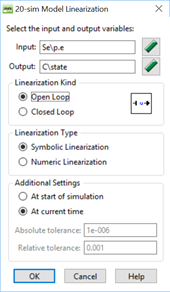
  2. From the Editor window, go to Tools, select Frequency Domain Toolbox, and then select Model Linearization. The 20-sim Model Linearization window opens, as shown in Figure 10‑5.

Figure 10‑5 Model Linearization interface in 20-sim

1. Select the input and output variables for which you want to draw the Bode plots. The resulting transfer function is related to this selection. Click on the Variable Chooser icon to get a list of model variables to choose from. Leave the rest of options as selected by default. Note that unless output is used as feedback, usually Open Loop is selected. Select OK.
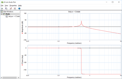
2. The 20-sim System Editor interface window opens (see Figure 10‑2). The transfer function, based on input/output selection appears. From the selections under Plots, choose the Bode The corresponding Bode plots appear in a new window as shown in Figure 10‑6.

Figure 10‑6 Typical Bode plots for a system

1. 1. Go to Properties and select Plots to edit plots for title, axes scales, labels, legends, etc.

1. Manual drawing of Bode plots using transfer function

1. Derive transfer function and transform it to $s$ -domain, $G(s)$ , using Laplace transform.
2. Plug in $s=j\omega$ into transfer function, to get $G(j\omega)$ .
3. Calculate the real and imaginary parts of the $G(j\omega)$ .
4. Calculate magnitude $|G(j\omega)|$ and power, using Equation (10.4).
5. Calculate the phase angle in degrees, using Equation (10.3).

Alternatively, Bode plots can be drawn using 20-sim after having the desired transfer function $G(s)$ from step 1 above, by following the guideline given in section 10.4.

10.5 Example: Bode Plots Using Transfer Function

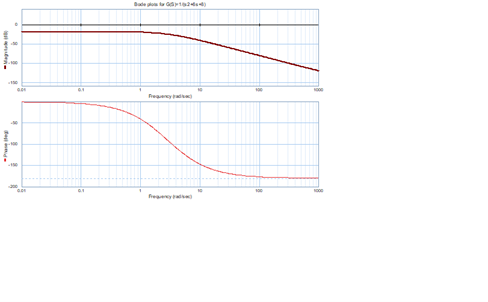
A system’s transfer function $G(s)=\dfrac{1}{s^{2}+6s+8}=\dfrac{1}{(s+2)(s+4)}$ is given. Find expressions for magnitude and phase angle and draw the corresponding Bode plots. Consider the frequency range 0.01–1000 rad/s. Discuss the system dynamical behaviour at low and high frequencies, including cutoff frequency.

Solution:

Using the guidelines, we substitute $s=j\omega$ in $G(s)$ . Therefore, $G(j\omega)=\dfrac{1}{(j\omega+2)(j\omega+4)}=\dfrac{1}{8-\omega^{2}+6j\omega}$ After multiplying and dividing by the conjugate of the denominator, we get $G(j\omega)=\dfrac{1}{8-\omega^{2}+6j\omega}\times\dfrac{8-\omega^{2}-6j\omega}{8-\omega^{2}-6j\omega}=\dfrac{8-\omega^{2}}{\omega^{4}+20\omega^{2}+64}-j\dfrac{6\omega}{\omega^{4}+20\omega^{2}+64}$ . From this expression, we get the real and imaginary parts as $\mathfrak{R}=\dfrac{8-\omega^{2}}{\omega^{4}+20\omega^{2}+64}$ and $\mathfrak{J}=-\dfrac{6\omega}{\omega^{4}+20\omega^{2}+64}$ . Using the real and imaginary parts and Equation (10.3), we can calculate the magnitude and phase as $|G(j\omega)|=\dfrac{1}{\sqrt{\omega^{4}+20\omega^{2}+64}}$ and $\varphi=\tan^{-1}(\frac{6\omega}{\omega^{2}-8})$ . Note that at $\omega=2\sqrt{2},\varphi=\pi/2$ and at $\omega=0,\varphi=\pi$ . We can draw the Bode plots, manually or using 20-sim, for example. The cutoff frequency can be calculated as follows. The gain magnitude at $\omega=0$ reads $|G(j\omega)|=\frac{1}{\sqrt{64}}=0.125$ . Therefore, the corresponding power is $20\log_{10}0.125=-18.0618\: dB$ . The cutoff frequency corresponds to $-18.0618+(-3)=-21.0618\:dB$ . Therefore, the corresponding gain is $G=0.0885$ , using $-21.0618=20\log{G}$ . After substituting for $G$ and using $G=\dfrac{1}{\sqrt{\omega^{4}+20\omega^{2}+64}}$ , we get cutoff frequency $\omega_{b}=1.672\:rad/s$ . The phase at the cutoff frequency can be calculated using $\varphi=\tan^{-1}(\dfrac{6\times1.672}{1.672^{2}-8})=-1.092\:rad$ or $\varphi=-62.57^{\circ}$ .

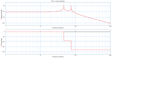
Following the steps given in section 10.4, we can use 20-sim and the transfer function $G(s)=\dfrac{1}{s^{2}+6s+8}$ to draw the Bode plots. The coefficients for the polynomials are (1) for numerator, and (1, 6, 8) for denominator. The resulting Bode plots are shown in Figure 10‑7.

The following video shows how to build and run the model for this example in 20-sim.

Figure 10‑7 Bode plots for the transfer function

10.6 Example: Bode Plots Using a BG Model

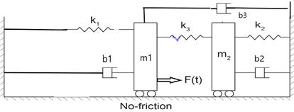
Build the BG model and its Bode plots considering transfer function based on force $F$ as input and displacement of the spring $k_{2}$ as output. Use the mechanical system as shown in Figure 10‑8 with

$m_{1}=20\:kg$ , $m_{2}=10\:kg$ , $k_{1}=35\:kN/m$ , $k_{2}=38kN/m$ , $k_{3}=15kN/m$ , $b_{1}=0.4\:N.s/m$ , $b_{2}=0.5\:N.s/m,$ $F=200\:N$ , and $b_{3}=0.1\:N.s/m$ .

The damper $b_{3}$ connects mass $m_{1}$ and the wall at the right side. Repeat the simulation for the following cases:

1. 1. Use given damper coefficient values $b_{3}=0.1,0.2,0.3,0.4,0.5,0.6 N.s/m$ to study its effect on the system with Parameter Sweep tool in 20-sim (available at the 20-sim Simulator window: select Tools > Time Domain Toolbox >Parameter Sweep). During the sweep, monitor the displacement of mass $m_{1}$ .
  2. Use a pulse-type signal as the applied force with amplitude 200 $N$ , start time 2 sec, and stop time 3.5 sec.

Figure 10-8 Mechanical system sketch for example given in section 10-6

Solution:

The following video shows how to build and run the model for this example in 20-sim.

Figure 10‑9 shows the resulting Bode plots. Note that in this video, the force is applied to mass $m_{2}$ , in the first try and then moved to mass $m_{1}$ according to the sketch shown in Figure 10‑8.