Bond Graph Models for Electrical Systems

Mehrzad Tabatabaian

7 Bond Graph Models for Electrical Systems

7.1 Overview

An electrical system may consist of components such as resistors, inductors, capacitors, transformers, and batteries/source. The generalized BG elements and relations apply to the analysis of dynamics of electrical systems and components in a similar way that the mechanical components were treated; i.e., they are analogous (see Table 3-1). In other words, electric charge $Q$ is equivalent to the generalized displacement $q$ , electrical current to $i=\dfrac{dQ}{dt}=\.{Q}$ to the flow $f$ , and voltage $V$ to the effort $e$ . The inductor (with inductance $L$ ) is analogous to point mass and is represented by $I$ -element; the capacitor (with capacitance $c$ ) is analogous to a mechanical spring and is represented by $C$ -element; and resistor (with resistance $R$ ) is analogous to mechanical damper and is represented by $R$ -element. The generalized momentum $p_E$ or flux linkage is the integral of $V$ with respect to time. Therefore, we can write

$\begin{equation*} \begin{dcases} e\equiv V, voltage\\ f \equiv i=\.{Q}, current\\ e \cdot{f} \equiv{V} \cdot{i}, power\\ q \equiv{Q}=\int\textit{i dt}, charge\\ p \equiv{P_E}=\int{V}{dt}, \textit{electrical momentum} \end{dcases} \end{equation*}$

Using the constitutive relations, for an $I$ -element we have $e=I\.{f}$ or $V=L\dfrac{di}{dt}$ , and for a C-element we have $e=q/c$ or $V=Q/c$ . Similarly, for an R-element we have $e=Rf$ or $V=Ri$ . The energy associated with storage elements can be written using Equations (3.7) and (3.8), or for elements I and C, as $\dfrac{1}{2L} p^2_E=\dfrac{L}{2} i^2$ and $\dfrac{1}{2c} Q^2=\dfrac{c}{2} V^2$ , respectively. An advantage of the bond graph method is its analogous applicability to different domains using the common constitutive relations, as described above for electrical systems.
The analogy between mechanical and electrical systems can be summarized as follows:

For a system with series-connected components, we have equal effort for mechanical and equal flow for electrical systems. For example, when a spring and a damper are connected in series, they experience the same force, and when a capacitor and a resistor are connected in series, they experience the same current.
For a system with parallel-connected components, we have equal flow for mechanical and equal effort for electrical systems. For example, when a spring and a damper are connected in parallel, they experience the same velocity (or rate of displacement), and when a capacitor and a resistor are connected in parallel, they experience the same voltage.

In other words, the relations of efforts and flows are swapped according to the type of the physical system between mechanical and electrical systems.

$\begin{multiline} mechanical|_{parallel} \: \equiv \: electrical|_{series}\\ \: \\ mechanical|_{series}\:\equiv \: electrical|_{parallel} \end{multiline}$

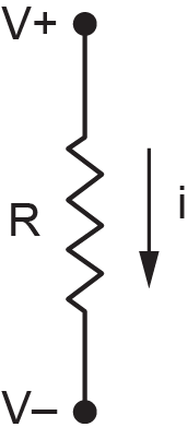
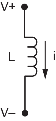
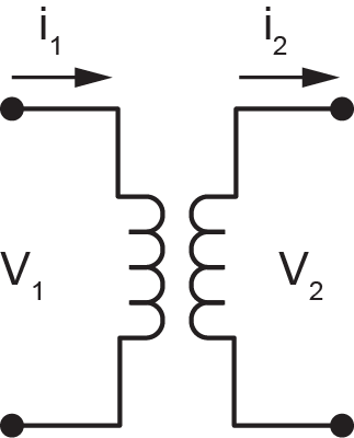
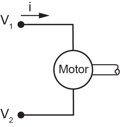
Table 7-1 shows typical components for resistor/ $R$ , capacitor/ $C$ , Inductor/ $I$ , Transformer/ $TF$ , Electric motor/ $GY$ .

Table 7‑1 Typical electrical components and their corresponding BG elements
$R$ -Element (resistor)	$C$ -Element (capacitor)	$I$ -Element (inductor)	$TF$ -Element (transformer)	$GY$ -Element (electric motor)

7.2 Example: Sign Convention for Electrical Systems

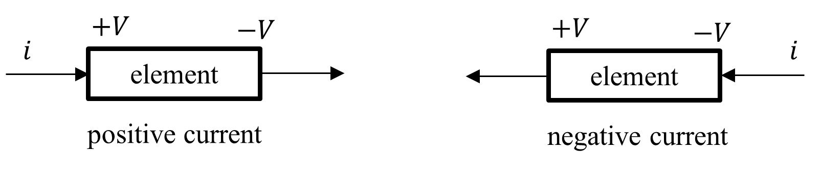
Like mechanical systems, for which we defined +C and +T sign convention for internal forces, we require to define a sign convention for electrical systems. It is customary to use the passive sign convention (PSC) for defining the direction of electrical current ( $i=\dfrac{dQ}{dt}$ ) passing through the elements of an electrical circuit. The background for the PSC is to have power being positive when absorbed by passive elements, e.g., $R$ -, $C$ -, and $I$ -elements in BG method. Therefore, for a typical passive element, by definition, the electrical current is considered as being positive when input into the element from its higher-voltage node (i.e., positive voltage/ $+V$ ) and output from the relatively lower-voltage node (i.e., negative voltage/ $-V$ ). Otherwise, the current is negative. See Figure 7‑1.

Figure 7-1 Sign convention for electrical current through passive elements, passive sign convention

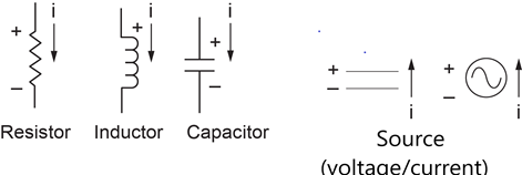
Using the PSC, we have power defined positive for positive current and negative for negative current, or $power=Vi>0$ when $V>0$ and $i>0$ ; hence, power is absorbed by the element. Otherwise, power is generated, when $\textit{power}=Vi<0$ when $V>0$ and $i<0$ . Figure 7‑2 shows the electrical power sign convention for passive elements ( $R$ , $C$ , $L$ ) and active elements (voltage and current sources).

Figure 7‑2 Electrical power sign for several elements according to passive sign convention

In the next section, we use the PSC for defining the current and voltage signs and discuss the step-by-step procedure for building BG models for electrical systems.

7.3 Guidelines for Drawing BG for Electrical Systems

As mentioned in chapter 4, the general guidelines for drawing BG model can be applied to electrical systems along with causality assignment rules. For electrical systems, we follow these guidelines, along with Kirchhoff’s circuit laws [24] and the PSC for building their BG models, as described in the following steps:

Assign voltage polarity ( $+V, -V$ ) for each element in the electrical circuit.
Assign current direction based on PSC for each element (see Figure 7‑1 and Figure 7‑2).
Assign 0-junction for each distinct voltage node in the circuit, according to Kirchhoff’s voltage law (KVL)—the algebraic sum of all voltage drops around a closed circuit is equal to zero.
Assign 1-junction for each element in the circuit, according to Kirchhoff’s current law (KCL)—the algebraic sum of all electrical currents entering and leaving a node is equal to zero). This is for taking care of relative voltage or drops related to each element located between two 0-junctions, since 1-junction is an effort summator.
Select a node in the circuit as a reference, i.e., the grounding, with zero voltage.
Assign $C$ -element for capacitors, $R$ -element for resistors, $I$ -element for inductors, $S_e$ for voltage, and $S_f$ for current sources.
Assign $TF$ -element for electrical transformers and $GY$ -element for electric motors.
Connect the elements with power bonds, assign causalities, and simplify by neglecting the bonds and the 0-junction which are connected to the ground source.

The above steps are based on KVL, and the process starts with assigning 0-junctions for each distinct voltage node. It is also possible to start with KCL and assign 1-junctions for the current in each closed-circuit loop and use 0-junctions in between for distribution of the current to corresponding circuit loops. The latter will result in a more simplified BG model and is recommended for complex circuits that involve several electric loops. In practice, we sometimes use a combination of these two approaches for building BG model for electrical systems.

In the following sections, we demonstrate the application of the procedure discussed above, with some worked-out examples.

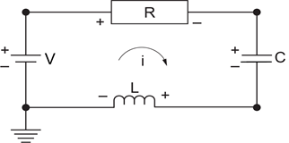
7.4 Example: An RCL Circuit—in Series

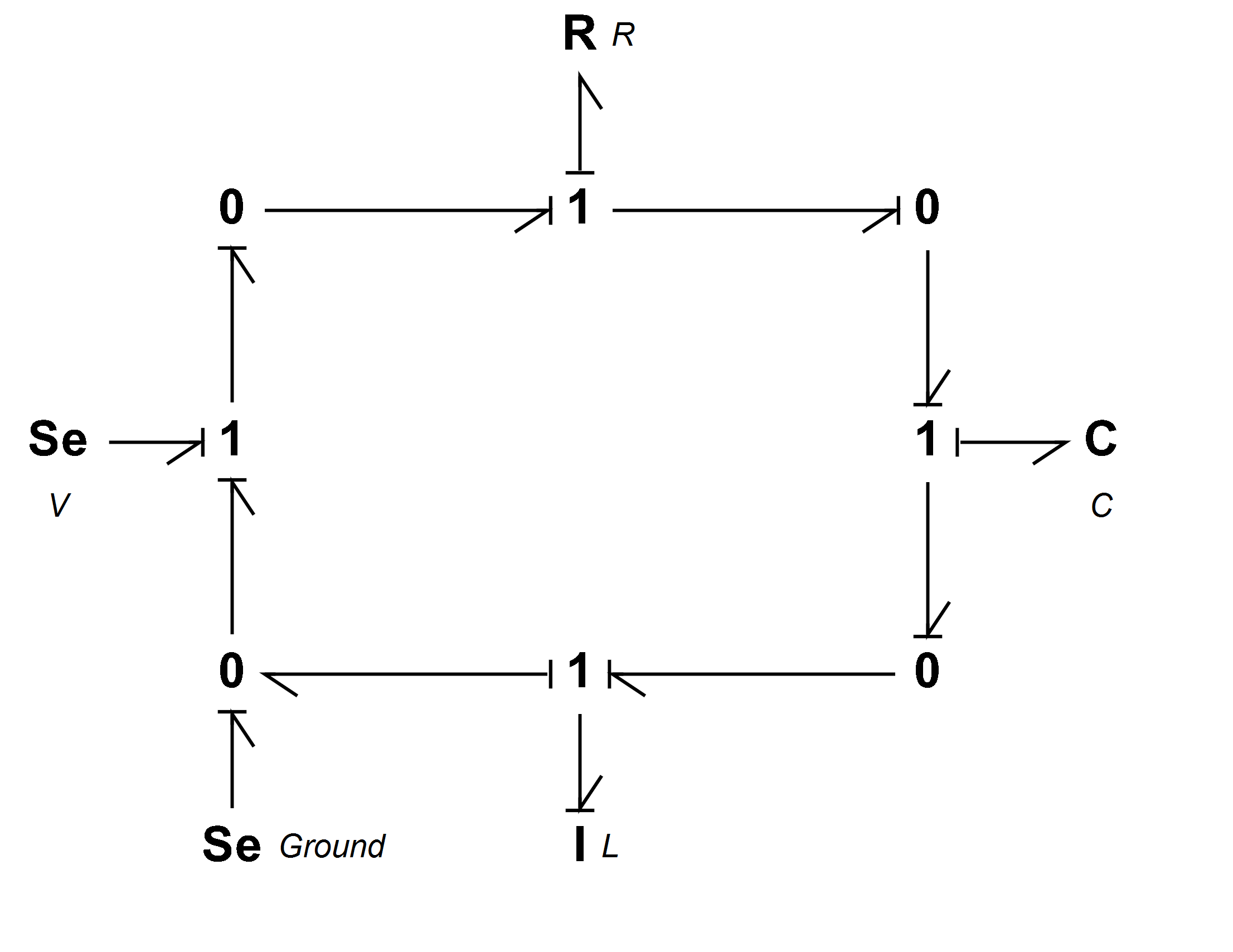
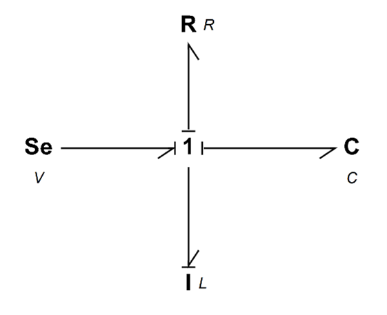
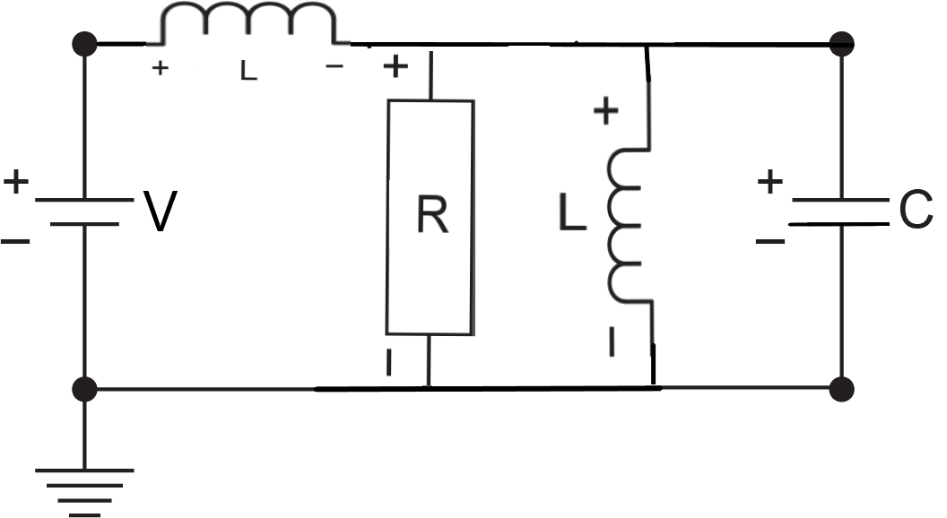
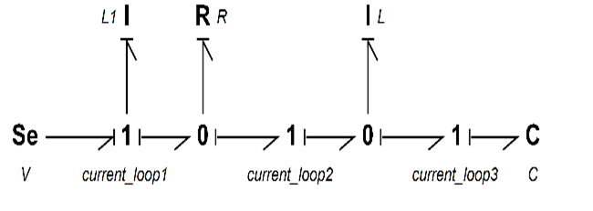
Figure 7‑3 shows an RCL circuit consisting of a resistor, a capacitor, and an inductor connected in series. To build the BG model, we apply the PSC and use the procedure listed in section 7.3. The four nodes identified by solid circles have distinct voltages. Therefore, four 0-junctions are assigned at the four corners of the circuit. For voltage drop across each element, we assign 1-juction and connect it to the corresponding element with a power bond. Note that the current direction in the circuit is consistent with the PSC convention. The resulting BG model is shown in Figure 7‑4 after being simplified with deleted ground-connecting bonds shown in the dashed circle. Alternatively, we can simplify the BG model and use a 1-juction for the current in the circuit loop according to KCL. In other words, the electrical current flowing through all elements should be identical. The resulting simplified BG model is shown in Figure 7‑5.

It is useful to discuss the analogy between the RCL circuit and mechanical mass-spring-damper systems (see Figure 4‑1) and their identical BG model. Assuming a ground connection for the circuit is analogous to a wall with zero velocity for the mass-spring-damper system, the current through the inductor is analogous to the velocity of the mass. The same current flows through the resistor and the capacitors, analogous to the velocity of the spring and damper components. Therefore, the simplified BG model (see Figure 7‑5) is identical for both electrical and mechanical systems. In other words, the BG model is identical to the one for a mass-spring-damper connected in parallel.

Figure 7-3 Sketch for a RCL electrical circuit in series

Figure 7‑4 BG model for a RCL electrical circuit in series

Figure 7‑5 Simplified BG model for an RCL electrical circuit in series

7.5 Example: An RCL Circuit—in Parallel

Figure 7‑6 shows an RCL circuit consisting of two inductors, a resistor, and a capacitor connected in parallel. We use the KCL approach to build the BG model for this example. Because the voltages across all components are identical, we can, using power bonds, apply a 0-junction (i.e., voltage equalizer) and connect the $R$ , $C$ , and $I$ components to it. This can be obtained by simplifying the BG model shown in Figure 7‑7.

Figure 7‑6 Sketch for a RCL electrical circuit in parallel

The following video shows how to build and run the model for this example in 20-sim.

Figure 7‑7 BG model for a RCL electrical circuit in parallel

7.6 Example: An Electrical Circuit—Two Loops

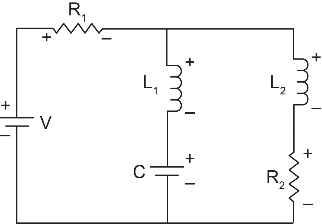
Figure 7‑8 shows an RCL two-loop circuit consisting of resistors, inductors, and a capacitor connected in parallel. We use the KCL approach to build the BG model for this example.

Figure 7‑8 A two-loop RCL electrical circuit

The following video shows how to build and run the model for this example in 20-sim.

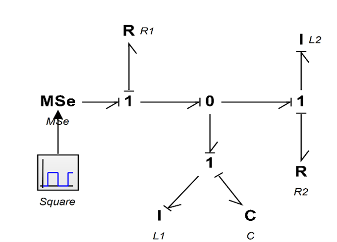
The simplified BG model with a supplied voltage signal as a square wave is shown in Figure 7‑9.

Figure 7‑9 BG model for the two-loop RCL electrical circuit

7.7 An Electrical Circuit—Three Loops

Figure 7‑10 shows an RCL three-loop circuit consisting of resistors, inductors, and a capacitor connected in parallel. We use the KCL approach to build the BG model for this example.

Figure 7‑10 A three-loop electrical circuit

The following video shows how to build and run the model for this example in 20-sim.

The simplified BG model with a supplied voltage signal as a block wave is shown in Figure 7‑11.

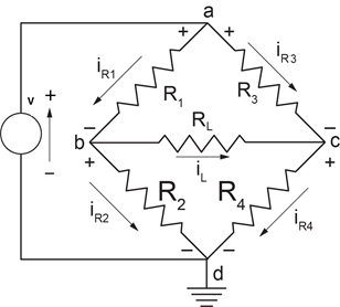
Figure 7‑11 BG model for the three-loop RCL electrical circuit

7.8 An Electrical Circuit—Wheatstone Bridge

Figure 7‑12 shows a Wheatstone circuit consisting of resistors. This circuit is usually used to measure an unknown resistor, e.g., placed in the system as $R_{4}$ , by adjusting the variable $R_{2}$ such that the current through $R_{L}$ is null, i.e., the balanced point. Using Kirchhoff’s and Ohm’s laws [25], we can calculate the currents going through the branch $abd$ as $\dfrac{V}{R_{1}+R_{2}}$ and branch $acd$ as $\dfrac{V}{R_{3}+R_{4}}.$ Therefore, the voltages at nodes $b$ and $c$ , with reference to the ground, are $V_{b}=\dfrac{V}{R_{1}+R_{2}}R_{2}$ and $V_{c}=\dfrac{V}{R_{3}+R_{4}}R_{4}$ , respectively. For having null voltage across $R_{L}$ , we let $V_{b}=V_{c}$ or after some manipulations, we get $R_{4}=\dfrac{R_{2}}{R_{1}}R_{3}$ . As shown, the balanced point is independent of the voltage supplied. We use the KCL approach to build the BG model for this example.

Figure 7‑12 A Wheatstone bridge electrical circuit

The following video shows how to build and run the model for this example in 20-sim.

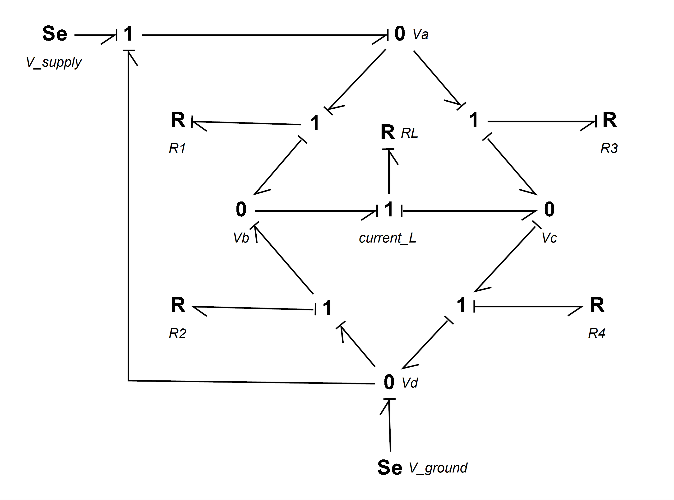
The simplified BG model with a supplied voltage is shown in Figure 7‑13.

Figure 7‑13 BG model for the Wheatstone bridge circuit

7.9 An Electrical Circuit—Multi-loop

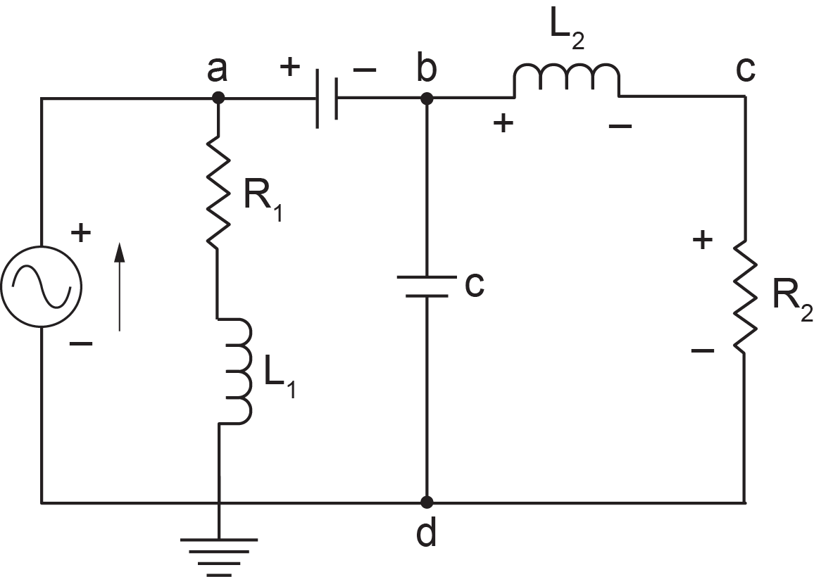
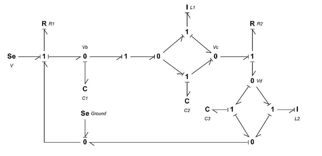
Figure 7‑14 shows an RCL multi-loop circuit consisting of resistors, inductors, and capacitors connected in series and parallel. We use the KCL/KVL approach to build the BG model for this example.

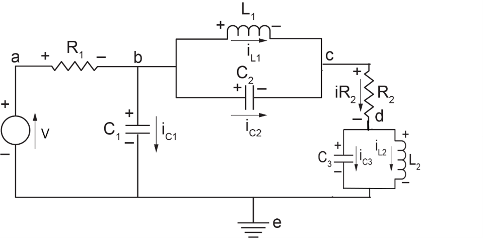
Figure 7‑14 A multi-loop electrical circuit

The following video shows how to build and run the model for this example in 20-sim.

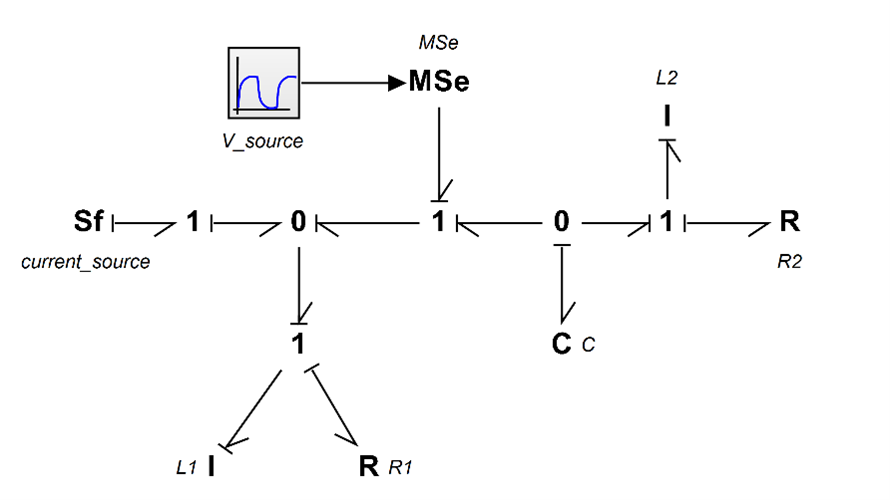
The simplified BG model with a supplied voltage is shown in Figure 7‑15.

Figure 7‑15 BG model for the multi-loop electrical circuit

7.10 An Electrical Circuit—Multi-loop with Transformer

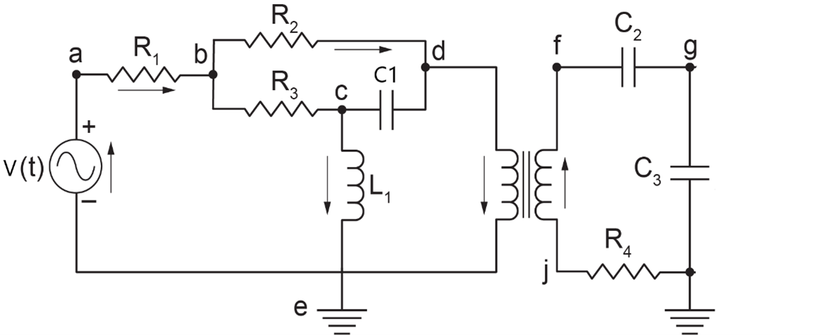
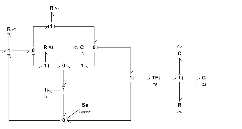
Figure 7‑16 shows an RCL multi-loop circuit consisting of resistors, inductors, capacitors, and a transformer connected in series and parallel. We use the KCL/KVL approach to build the BG model for this example.

Figure 7‑16 A multi-loop electrical circuit with transformer

The following video shows how to build and run the model for this example in 20-sim.

The simplified BG model with a supplied voltage is shown in Figure 7‑17.

Figure 7‑17 BG model for the multi-loop electric circuit with transformer

Exercise Problems for Chapter 7

Exercises

Build the BG model for the electrical system as shown in the sketch. Run the model and report the following quantities:
1. charge accumulated on capacitors
2. current across resistors
3. voltage drop across resistor $R_2$
4. momentum (flux linkage) for the inductor.

Use following data: $V(t)=100\sin(20t)$ , $R_1=0.1k\Omega$ , $R_2=0.5k\Omega$ , $R_3=0.8k\Omega$ , $C_1=200\mu{F}$ , $C_2=400\mu{F}$ , $L_1=5mH$ , and transformer parameter 2:1. Perform Parameter Sweep on a range of $TF$ parameter values, 0.5-3 and graph the results for electric charge on capacitor $C_2$ .

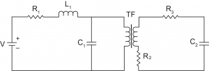
Build a BG model for the electrical circuit shown. Use $R=3k\Omega$ , $C=1\mu{F}$ , $L=100mH$ for simulation. Report voltages across each element for a direct source voltage of $5V$ . Also, run the model for a range of capacitance $10nF$ , $100nF$ , $1000nF$ using Parameter Sweep and report the across the inductance for these values. Draw the sketch.

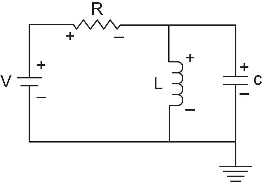
For the electrical system shown in the sketch, build the BG model.

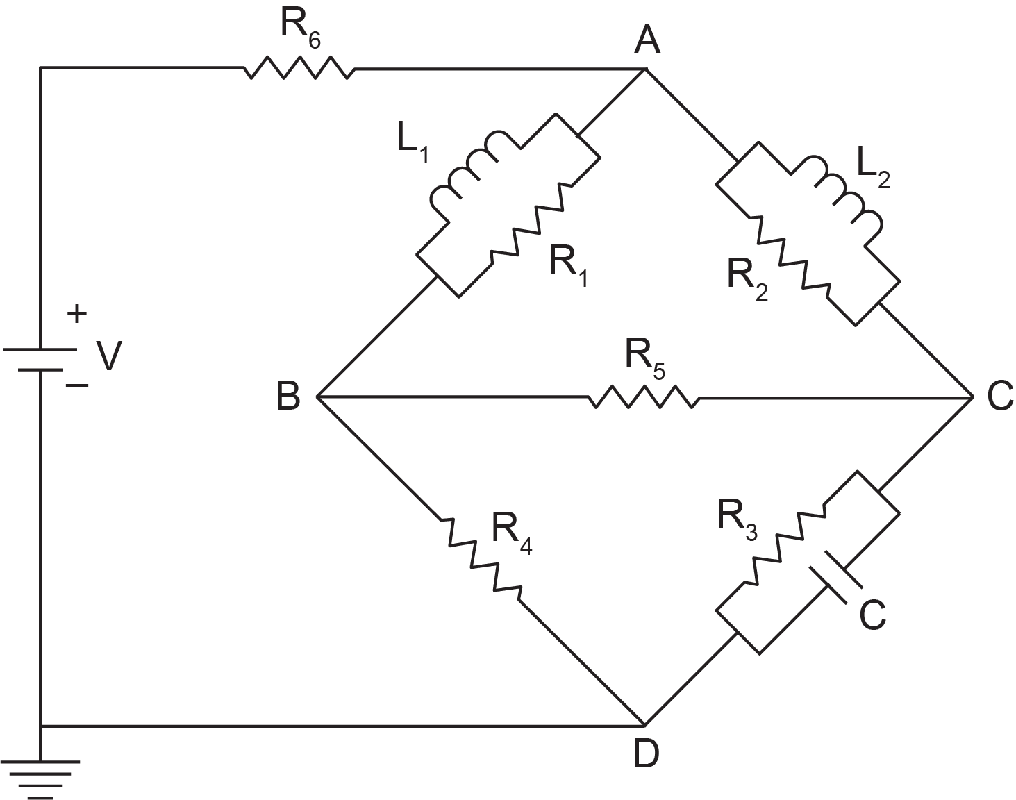
A modified Wheatstone bridge circuit is shown in the sketch. Build a BG model and show that the voltage across the bridge resistor (R5) is null when the bridge is balanced.

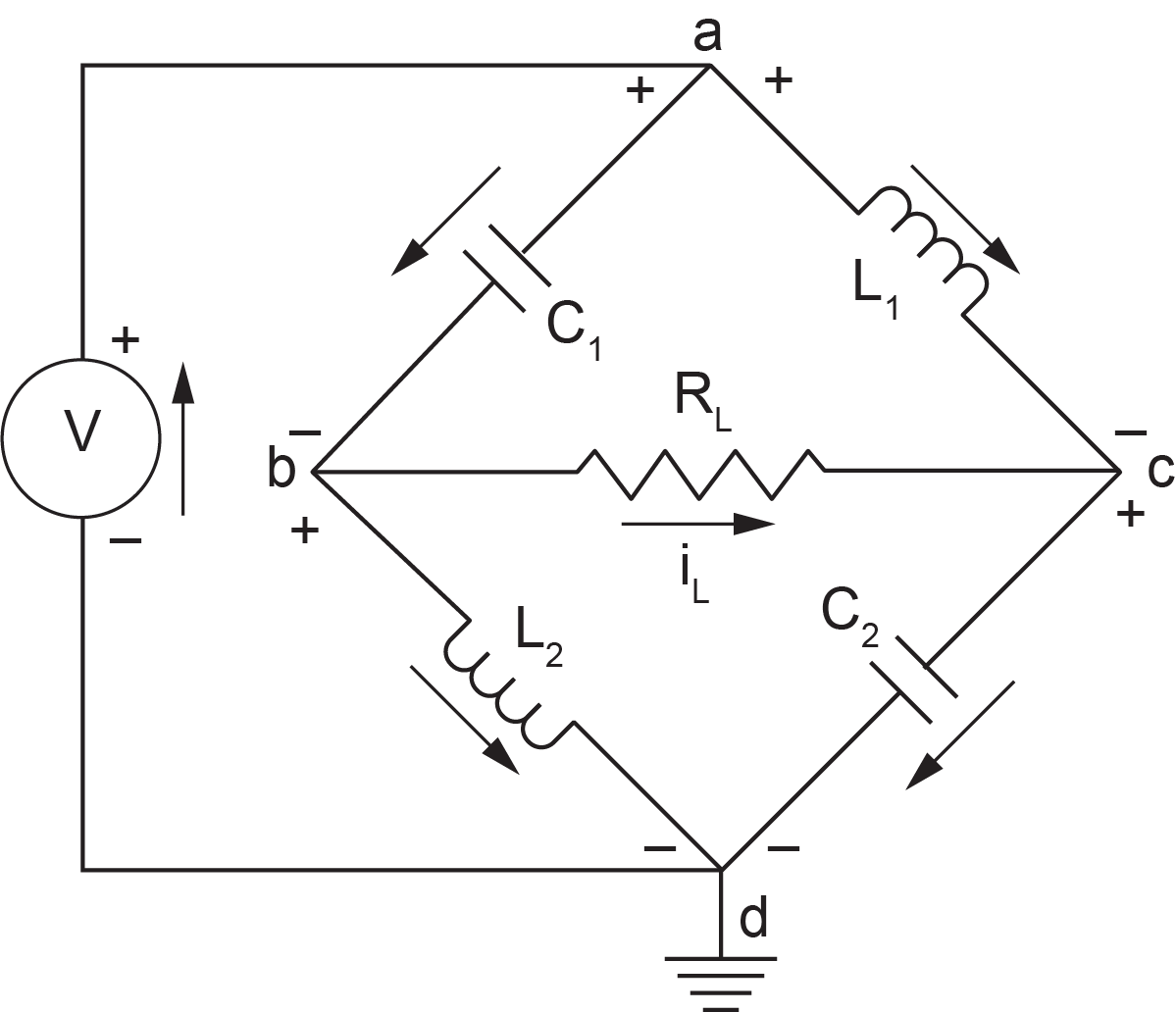
An electrical circuit is shown in the below sketch below. The circuit consists of two capacitors, two inductors, and one resistor. Build the corresponding BG model.

Modify the example given in section 7.7 by making the components branching from node $a$ to be laid out in parallel. Build the BG model for the modified circuit.
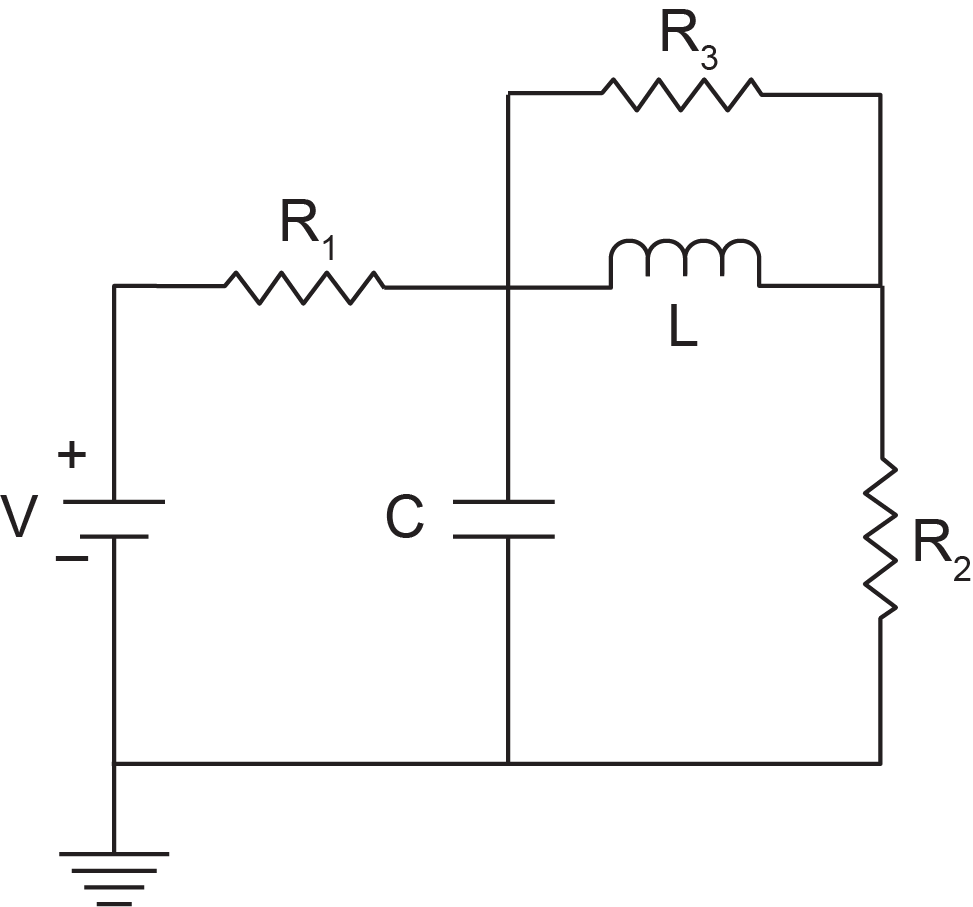
For the example given in above section 7-9, use the corresponding BG model and the following data to simulate the system: $V(t)=60\sin(15t)$ , $R_1=0.1k\Omega$ , $R_2=0.5k\Omega$ , $C_1=200\mu{F}$ , $C_2=400\mu{F}$ , $C_3=300\mu{F}$ , $L_1=5mH$ , $L_2=10mH$ .
Build the BG model for the electrical circuit shown below. After building the model in 20-sim, simplify it and interpret the simplified model. Perform a parametric sweep analysis for the capacitor and inductor.