4.1        Overview

To demonstrate applications of BG method, we discuss the procedure for building BG models for physical systems, using the material presented in chapter 3. We use examples related to mechanical systems to establish the guidelines and steps required to build a BG model. In further chapters, we present more worked-out examples for several engineering systems and disciplines, including electrical, hydraulic systems.

4.2        Steps for Building Bond Graph Models: General Guidelines

As mentioned, BG method can be used to build models for single- and multi-domain physical systems. The building blocks are the nine basic BG elements, including their modulated versions, and causality assignment rules (see section 3.4). A model for any specific system also requires definitions of relevant sign conventions for general displacement and forces. This chapter will discuss the latter and will present some worked-out examples. The following are the steps for building a BG model, in general, including for mechanical, electrical, and hydraulic systems:

1. Identify the physical system components in terms of their type (energy storage, source, dissipater, etc.).
2. Identify the DOF (degrees of freedom) of the system. This step is optional but recommended.
3. Identify and list the required BG elements.
4. Identify distinct physical points/nodes of the physical systems:
   • velocity or force (mechanical systems): translational
   • angular velocity or torque (mechanical systems): rotational
   • voltage or current (electrical systems): electrical circuits
   • pressure or flow rate (hydraulic systems): fluid network
5. Assign proper BG multi-port junction elements^[1] to items from step 4:
   • “1” for velocity, angular velocity, and electrical and flow currents
   • “0” for force, voltage, and pressure
6. Connect associated elements, using BG elements and power bonds, to the items from step 5.
7. Assign proper BG multi-port junction elements in between those items from step 5:
   • “0” for relative velocity and angular velocity
   • “1” for voltage drop and pressure drop
   • and for energy conversion
8. Connect associated elements to items from step 7, using BG elements and power bonds.
9. Define sign convention and connect all remaining power bonds.
10. Apply all causality assignments (integral causalities must be given priority).
11. Draw and build the BG model in 20-sim (when available).
12. Perform simulation and design, using the obtained BG model (when required).

In further sections, we will demonstrate implementation of the procedure/algorithm mentioned above with some worked-out examples, including power bond direction, causality assignment, and sign convention.

4.2.1        Guidelines for Power Bond Direction

Connecting elements in a BG model with power bonds requires compliance with the direction of energy flow in the physical system. Therefore, the directions of half-arrows are critical. The following guidelines may be helpful:

1. Draw power bonds from BG source elements ( and ) toward the system, connecting to the adjacent elements.
2. Draw power bonds toward BG passive elements (i.e., , , and )
3. Draw power bonds to and from BG junction elements (“1” and “0”) according to a previously defined sign convention (see section 3.4.5).
4. Draw remaining power bonds to have all BG elements connected.
5. Some simplifications of the BG model may be justified, but not required.

After drawing all power bonds for the model, assign the causality strokes. The next section provides a list of guidelines for causality assignments.

4.2.2        Guidelines for Assigning Causality Strokes

The assignment of causality strokes is a required step in building any BG model. The following steps help with achieving this requirement.

1. Assign causality to BG source elements.
2. Assign causality assignments with preferred integral causality strokes to – and – elements.
3. As far as possible, extend the causality assignments to other power bonds, using the causality requirements for connecting elements (e.g., 1, 0, and )
4. Assign causality assignments to -elements that accept neutral causality stroke assignment.
5. As far as possible, using the causality requirements for connecting elements, extend the causality assignments to all remaining power bonds in the model.

If execution of step 5 from the above list cannot be completed, then the BG model contains some specific mathematical properties—algebraic loop or differential/derivative causality (see chapter 11). The application 20-sim automatically assigns the causality strokes with prioritizing integral causalities, and if present, identifies the derivative or algebraic loops causalities in the model with red-colour strokes. In further sections, we will explore these features, with some examples.

4.3        Example: BG Model for a One-DOF Mass-Spring-Damper Mechanical System

A mechanical system consists of mass [kg], spring [N/m], and damper [N.s/m]. The applied force on mass is . Build a BG model for this system as shown in Figure 4‑1, neglecting friction of the rollers.

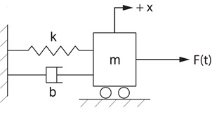
Solution:

DOF = 1 (1D translational motion of one mass) and the required BG elements are: (representing the mass), (representing the spring), (representing the damper), (representing force ) and (representing the wall velocity). Also, we are required to have junctions “1” and “0.”

1. Distinct velocity nodes are the mass and the wall (although the wall usually is stationary). Hence, we need two “1” junctions to represent common velocity for all elements attached to the mass and the wall.

We draw them as

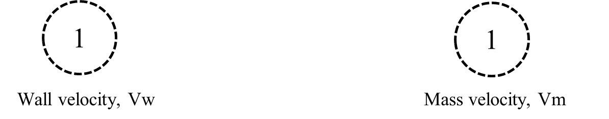
As well, for each junction, it is useful to assign a name related to its representation.

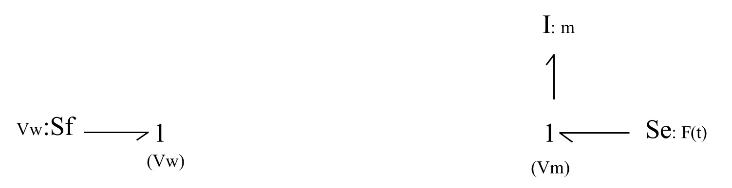
2. We draw all elements connecting to the junctions which have the same distinct velocity values and connect them with power bonds. Therefore, for the wall-velocity junction, we use flow source and for mass-velocity junction and inertial element , representing the mass and a representing the applied force Note that -element should receive power (passive element), and sources send power to the system (active elements).

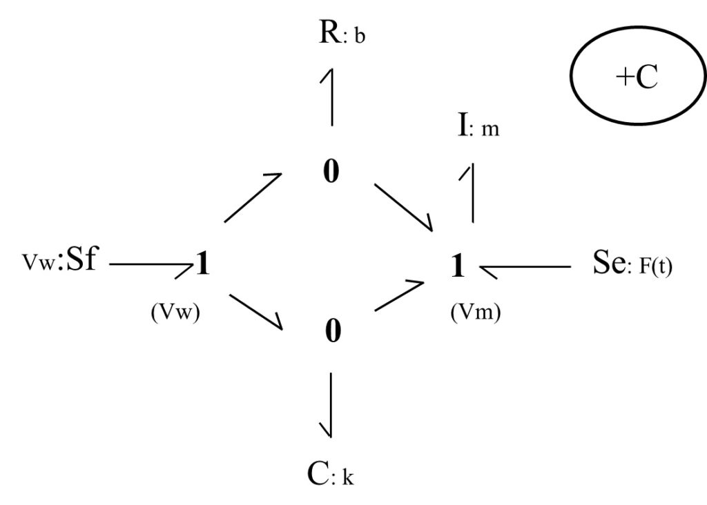
3. The spring and damper experience the same value of relative velocity, ||, which is represented by 0-junctions. Recall that 0-junction element is a flow summator. According to the power bonds connecting the spring (or damper) to the 0-junction, we can have () or (), considering the -coordinate as given in Figure 4‑1. Therefore, to specify the associated power bond directions we should define a sign convention. The common practice is to consider the spring (or damper) from the BG model and define either tension force as being positive (+T) or the compression force being positive (+C). For this example, we use the spring displacement/velocity to demonstrate the sign convention. A similar argument applies for the damper’s displacement.

To represent the relative velocity, we add two 0-junctions and – and – elements to the model and use, e.g., (+T) sign convention, as shown below:

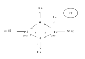Note that – and – elements are passive and should receive power from the system. After labelling the bonds connecting to the 0-junction associated with the – element, we can write the power balance as . But . Hence, , or where is the spring displacement rate or velocity equal to the relative velocity. Now, to have the displacement of the spring in the + direction, we should have or . This implies that the displacement/velocity of the mass should be larger than that of the wall, for the spring is experiencing a positive tension force. Therefore, the spring is under tension and the assigned sign convention (+T) is satisfied, considering the + direction.

Now, if we change the power direction of the bonds connecting to the 0-junction, as shown in the sketch below, we have , or ; hence, we have the spring under compression. Therefore, the (+C) sign convention is satisfied. Note that only the power direction of the four bonds associated with the two 0-juctions can change their directions since the rest are associated with source or passive elements and are unique in their directions, as shown below. 

Both sign conventions are legitimate, but only one should be selected and used consistently for building a BG model. We continue, using the BG model with (+T) sign convention.

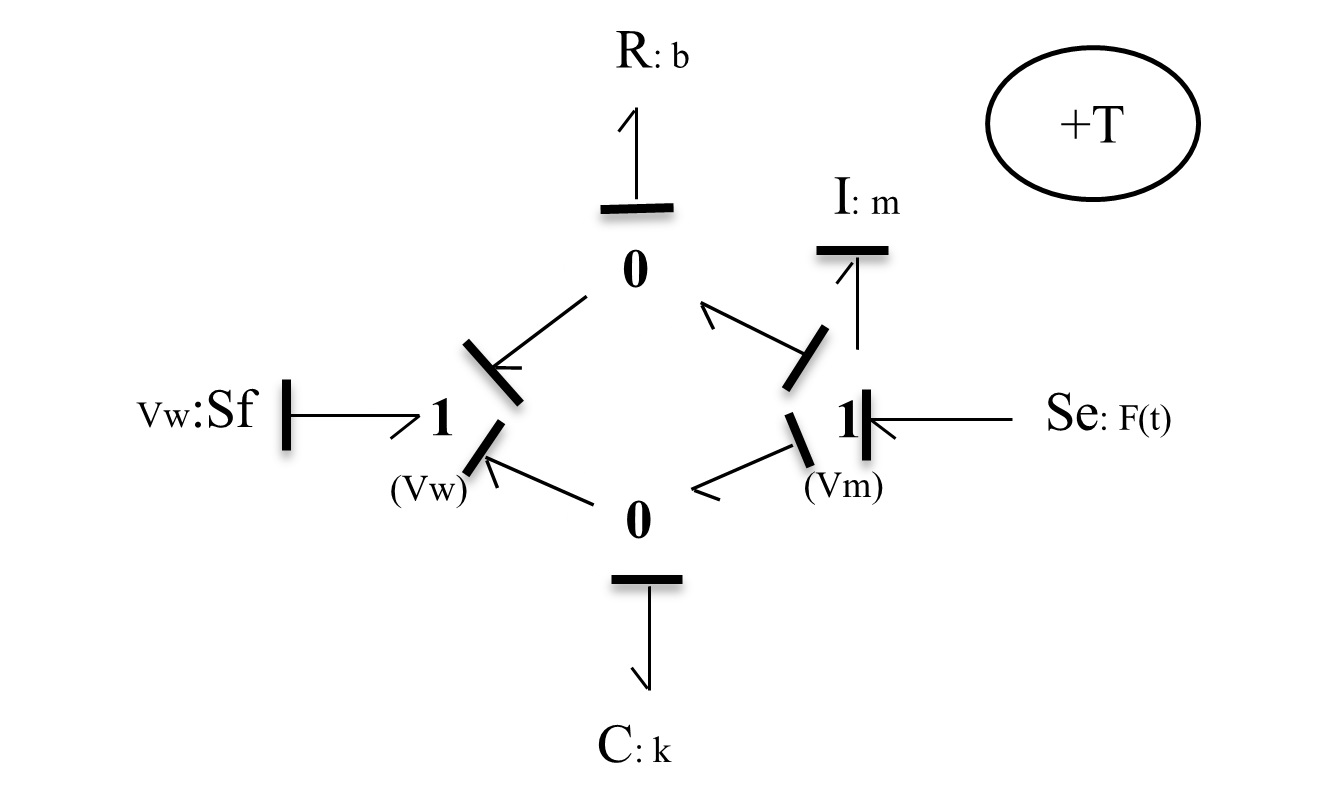
4. Causality assignments are now applied, according to the rules discussed in chapter 3. Following the guidelines given in section 4.2.2, we start applying the causality to the source elements, followed by those for – and – elements. Recall that integral causalities are preferred for elements (i.e., receives effort) and (i.e., C sends effort). The causality strokes are shown with transvers lines, as shown below.

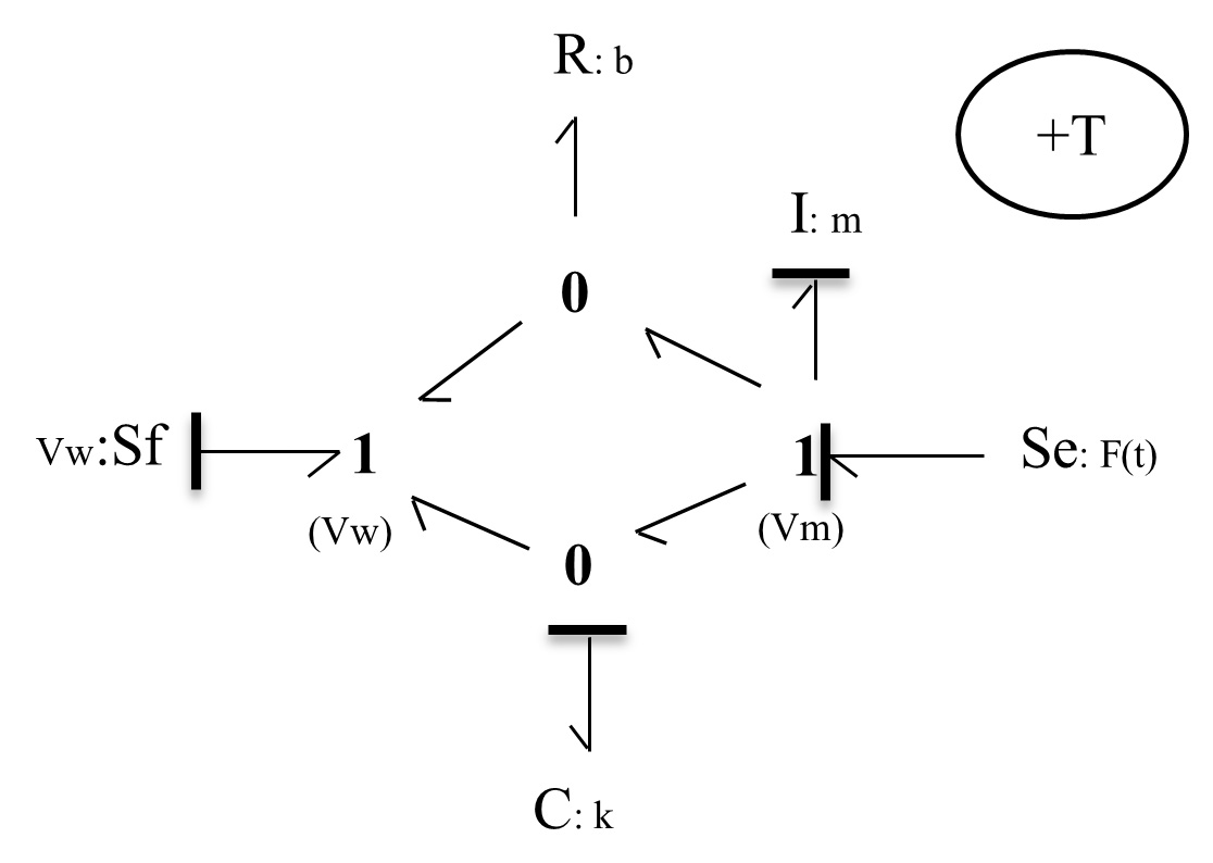
5. Extend the causality assignments to the remaining bonds, using the rules for 1-junction (can receive only one flow signal through its strong bond) and 0-junction (can receive only one effort signal through its strong bond), as shown below in the model sketch (see Figure 4‑2).

 

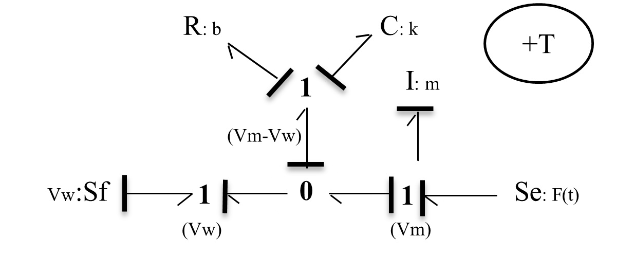
6. To a reasonable extent, we can simplify the BG model such that it clearly resembles the physical system. The two 0-junctions represent the same value of relative velocity, . Therefore, we can combine them into a single 0-junction and share the relative velocity value through a 1-junction element with the – and – elements. This simplification becomes very useful for building large BG models for more complex systems. Figure 4‑3 shows the resulting BG model. Note that the causality strokes should be adjusted after simplifications are made.

4.4        Example: BG Model for a Two-DOF Mass-Spring-Damper Mechanical System

Build the BG model for the mechanical system as shown in Figure 4-4. Consider the (+C) to be the sign convention for internal forces.

 

 

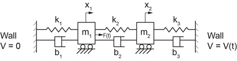
Solution:

This system has two DOF and four distinct velocity points, corresponding to mass and and the two walls. Therefore, we lay out four 1-junctions to represent them in the model. The remaining required BG elements are , , , , , and 1- and 0- junctions.

We follow the same guidelines demonstrated in the previous example (see section 4.3) and build the BG model as shown in Figure 4-5.

 

 

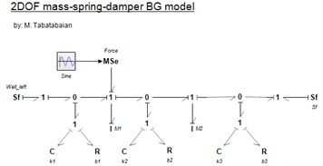
The reader is encouraged to build this BG model and to compare the results with those provided in Figure 4-5. The 20-sim BG model and a screen recording are available as companion resources describing the process to build the equation model and typical results for this example.

4.5        Example: BG Model for a Three-DOF Mass-Spring-Damper Mechanical System

Build the BG model for the mechanical system as shown in Figure 4-6. Consider the (+C) to be the sign convention for internal forces.

 

 

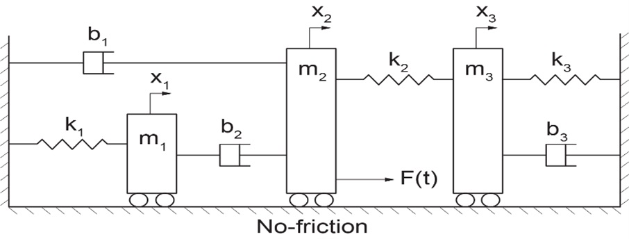
Solution:

This system has three DOF and five distinct velocity points corresponding to mass , , and and the two walls. Therefore, we lay out five 1-junctions to represent them in the model. The remaining required BG elements are , , , , , and 1- and 0-junctions.

We follow the same guidelines demonstrated in the previous example (see section 4.3) and build the BG model, as shown in Figure 4-7.

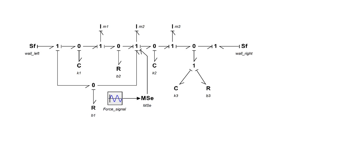
The reader is encouraged to build this BG model and compare the results with those provided in Figure 4-7. The 20-sim BG model and a screen recording are available as companion resources describing the process to build the equation model and typical results for this example.

4.6        Example: Kinetics and Kinematics of a Mechanical System Using BG Model

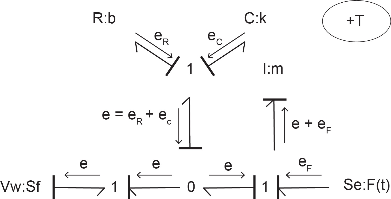
As mentioned previously (see section 3.2), one of the advantages of BG modelling method is that a BG model allows us to gain insights by visual inspection of the BG model. This can be achieved by drawing the streams of efforts (kinetics) and flows (kinematics) for a BG model.

In this example, we use the results from the example given in section 4.3 to demonstrate this property by explicitly drawing the effort and flow associated with each power bond in the model. First, we look at the kinetics of the system by drawing the efforts, as shown in Figure 4-8. As shown, the efforts/forces associated with the spring and dumper are collected as force and transferred to the mass in addition to the applied force shown as . Clearly, the wall receives the collected force .

 

 

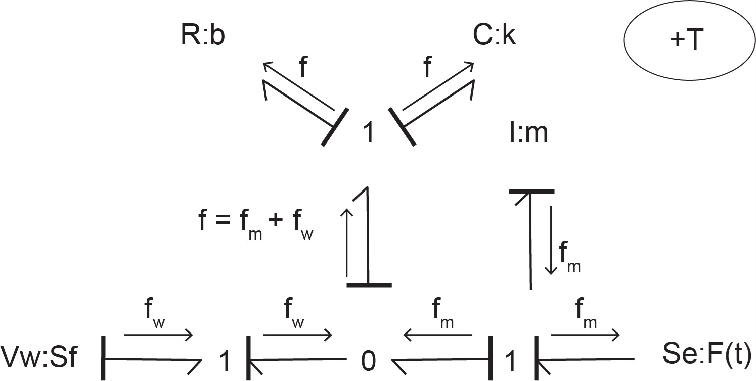
Similarly, by drawing the flows, as shown in Figure 4-9 the kinematics of the system can be visualized. As shown, the flows/velocities associated with the mass and wall are collected as velocity and transferred to the spring and damper. Clearly, these elements receive the relative velocity due to the motion of mass and the wall (if stationary, ).

 

4.7        Modelling and Simulation Approaches in Engineering: Modern vs. Traditional

Considering BG—our focus in this textbook—as the modelling method, once we have the corresponding BG model, we can proceed to simulation, and hence, design of a system. One can take two approaches to perform this task: traditional or modern. As mentioned, the main objective of modelling and simulation is to help with more effective design of the systems in terms of their cost, function, material consumption, etc. Therefore, any modelling method, including bond graph, should result in a mathematical model consisting of the systems’ equations. The solution of the equations can be used for system simulation and analysis to support effective system design. In the following sections, we briefly describe possible approaches and the reason for choosing the modern approach over the more traditional one.

 

4.7.1        Traditional Approach

Once the BG model is available for a system, we can derive/extract the system equations from the BG model—usually a laborious task—and then using numerical methods, we can obtain their solutions. This task is usually achieved with the help of computer programs (usually developed from scratch) based on a selected numerical method. This approach, along with both its system equation extraction and especially the computer coding, is limited in practical application, being specific from one problem to another one, and is laboriously time consuming. Figure 4-10 shows the major steps of the traditional approach.

 

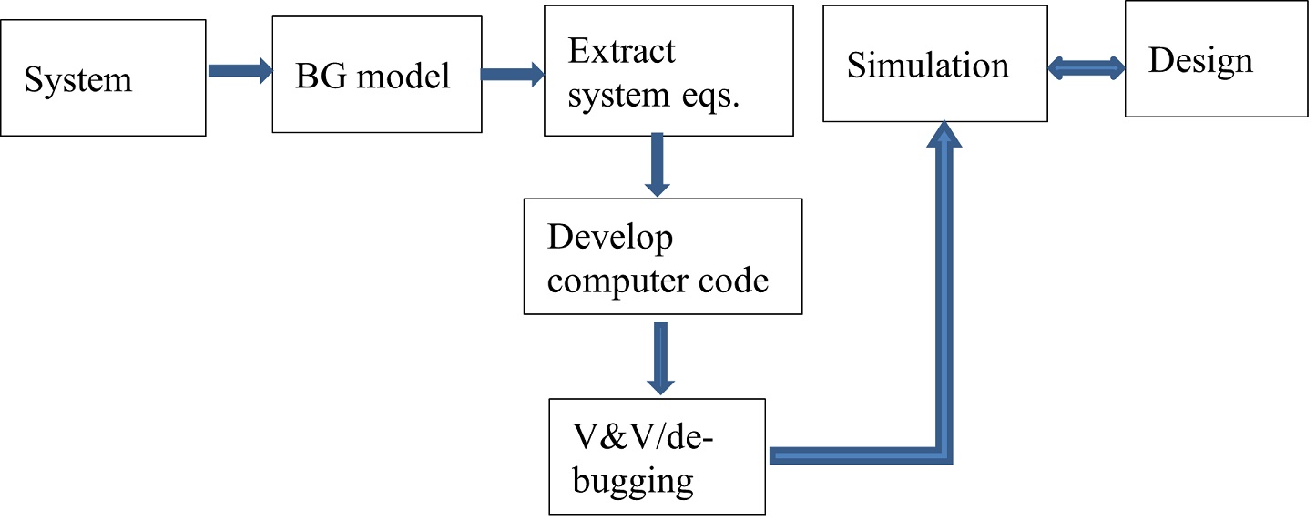
In practice, it is inefficient to develop computer codes for each specific design: the amount of person power, computer power, and other resources become overwhelming for the fast-paced engineering design needs of today’s industries. Therefore, a huge effort has been made to develop commercially available software tools to help meet these objectives and to make the whole process of system design more effective, economically viable, and efficient.

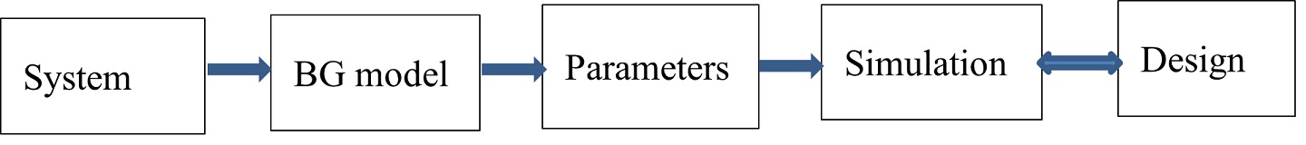
4.7.2        Modern Approach

Alternatively—or rather, preferably—the modern approach in engineering and system design employs related software tools. These tools provide opportunities to perform systems simulation immediately after obtaining the BG model. The software tool that we introduce and use in this textbook, 20-sim, helps with extracting the system equations from the BG model seamlessly and provides facilities for system simulation and parametric analysis. This modern approach is more effective in engineering practice and provides more and quicker insights into engineering systems design. In addition, the modern approach helps to respond more effectively to the fast-paced engineering demands in industry and is recommended for engineers in practice. Figure 4-11 shows the major steps of the modern approach. Note that verification and validation should be considered in the modelling step as well.

 

In the next section, we introduce the 20-sim software package with a focus on bond graph modelling, simulation, and time and frequency analysis for engineering systems and design. In further sections, we use 20-sim to build BG models and their simulations and to study their dynamical behaviour.

Exercise Problems for Chapter 4