8 Bond Graph Models for Hydraulic Systems
8.1 Overview
The generalized BG elements and relations apply to the modelling of dynamics of hydraulic systems in a similar way that the mechanical or electrical systems were treated; i.e.; they are analogous (see Table 3‑1). In this chapter, we define the effort and flow for hydraulic systems and derive the relations for hydraulic capacitance, inertance, and resistance corresponding to BG elements  ,
,  , and
, and  , respectively. Note that the complexity of fluid behaviour in static or dynamic flow conditions require us to pay more attention to identify these quantities and relations as compared to those for mechanical and electrical systems.
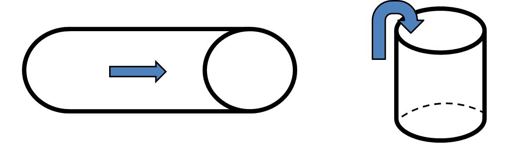
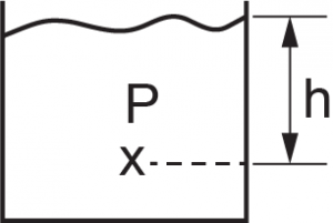
For modelling hydraulic systems, we are usually interested in having a relationship between pressure and fluid volume in static conditions and between pressure drop and fluid volume flow rate in dynamic conditions. For example, we might be interested to know the pressure drop for a given flow rate in a pipe, or we might want to know the pressure at a given depth in a storage tank, as sketched in Figure 8‑1.
8.2 Definitions of Effort, Flow, and Momentum for Hydraulic Systems
Recall that power is the quantity of interest in BG method (see section 3.2). Considering a control volume  of an incompressible fluid flowing under pressure
  , we can write the power
  as the product of the force
  exerting on the fluid, resulted from applied pressure, and the velocity
  of the fluid flowing through the volume, or
  But the velocity of the fluid can be written as
  , using the continuity relation, where
  is volume flow rate of the fluid and
  is the cross-sectional area of the control volume. Therefore, after substitution, we get
  , or equivalently rate of energy
  . Comparing the relation
  with the BG generalized relation for power, i.e.,
  , we can write
  and
and  . In other words, for hydraulic systems, pressure is equivalent to BG effort, and fluid volume flow rate is the BG flow. Similarly, we can write the generalized BG displacement
  as the volume of the fluid, or
  .
.
In BG method, the generalized momentum is the integral of effort. Therefore, we can write the fluid momentum  as the integral of pressure, or
  . Summarizing these relations, we have

8.3 Fluid Compliance: C-element
Fluid compliance or hydraulic capacitance describes potential energy storage with a fluid, e.g., the height of fluid in a tank. It is equivalent to mechanical spring compliance or electrical capacitor capacitance. For a -element in BG method, we have  . Using equivalent quantities for hydraulic systems, we can write
  , or fluid compliance is volume change per unit of pressure acting on the fluid volume. For an incompressible fluid with density
  , the hydrostatic pressure at depth
  is
is  and the volume of the fluid is
  . After substitution, we get
  , or after rearranging and simplifying, the hydraulic capacitance for incompressible fluid is
(8.1) 
where  is the gravitational acceleration. The dimension of fluid compliance can be worked out as
 ![[\dfrac{m^4s^2}{kg}]](https://pressbooks.bccampus.ca/engineeringsystems/wp-content/ql-cache/quicklatex.com-d754f821dd0f3326a4d2bd869614763b_l3.png "Rendered by QuickLaTeX.com") = [
= [ ] =
] =  .
.
Note that the pressure could be replaced by total dynamic pressure for fluid in motion.
If the fluid is compressible, we use the bulk modulus of elasticity  for calculating the change in volume. By definition, is pressure needed to change fluid volume per unit of volume, or
  . Therefore,
  .
.
(8.2) 
For more complex flow and non-uniform, flexible tubes, consult with chapter 4 of Dean, Karnopp, Margolis, and Rosenberg [20].
Having the hydraulic capacitance, we can write the relation between the flow rate and the pressure as  , useful to calculate the flow rate for given pressure. Similarly, we can write
  , useful for calculating pressure for given flow rates.
(8.3) 
Note the similarity between relations given by Equation (8.3) and those given for mechanical spring (when pressure is replaced by force and fluid volume flow rate by velocity) and electrical capacitance (when pressure is replaced by voltage and fluid volume flow rate by current).
8.4 Fluid Inertia: I-element
Fluid inertia, or hydraulic inertance, describes kinetic energy storage with a fluid or the inertia, e.g., of a fluid flowing in a pipe. It is equivalent to inertia related to mass in mechanical or inductance in electrical systems. For an -element in BG method,  describes the relation between generalized momentum and flow. Using equivalent quantities for hydraulic systems, we can write
  , or fluid pressure momentum is the product of fluid inertia by its volume flow rate. To derive the relation for , we require to have the relationship between the momentum and volume flow rate of the fluid flow. For derivation, we consider a control volume with length
  and cross-sectional area of the fluid with density , as shown in Figure 8-2.
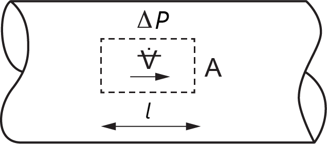
Assuming a pressure difference  between two ends of the control volume acting on the fluid, we can write Newton’s second law for the fluid motion as
 . Rearranging the terms and integrating the pressure, we get the pressure momentum
  . But volume is
  . After substituting, we get the relationship between pressure momentum and the volume flow rate as
(8.4) 
Comparing Equation (8.4) with the generalized momentum equation for -element, we can write the fluid inertia as
(8.5) 
The dimension of fluid inertia can be worked out as ![[\,\dfrac{kg}{m^4}]\, \equiv \dfrac{pressure\: momentum}{volume\: flow \:rate}](https://pressbooks.bccampus.ca/engineeringsystems/wp-content/ql-cache/quicklatex.com-d3751e078f0411692978b639f2e18e3c_l3.png "Rendered by QuickLaTeX.com") .
.
From Equation (8.5), we can conclude that a fluid has larger inertia when flowing in small diameter tubes, compared to in larger tubes because is inversely proportional to . This effect is counterintuitive and is sometimes misinterpreted with the wrong assumption that large-size tubes should exhibit larger inertia effects. Note that we consider only force due to pressure, and not friction due to viscosity, assuming an ideal fluid.
For more complex flow and non-uniform and/or flexible tubes, consult with chapters 4 and 12 of Dean, Karnopp, Margolis, and Rosenberg [20]. For example, if the cross-section of the pipe and the density of fluid change along its  -axis, then we get
(8.6) 
Having the hydraulic inertance, we can write the relation between the flow rate and the pressure as  , useful to calculate the flow rate for given pressure. Similarly, we can write
  , useful for calculating pressure for given flow rates.
(8.7) 
Note the similarity between relations given by Equation (8.7) and those given for mechanical systems (when pressure is replaced by force, fluid flow rate by velocity, and inertance by mass) and electrical systems (when pressure is replaced by voltage, fluid flow rate by current, and inertance by inductance).
8.5 Fluid Resistance: R-Element
Fluid, or hydraulic, resistance describes energy dissipation with a fluid, e.g., friction of a fluid flowing in a pipe. Fluid resistance is equivalent to dampers in mechanical or resistors in electrical systems. For an -element in BG method, we have  Using equivalent quantities for hydraulic systems, we can write
(8.8) 
or fluid resistance is equal to pressure change per unit volume flow rate. This relationship depends on the state of the flow (e.g., laminar, turbulent) and the fluid properties (e.g., ideal, viscous,) [26], [27], [28]. Note the similarity between relations given by Equation (8.8) and those given for mechanical systems (when pressure is replaced by force and fluid flow rate by velocity) and electrical systems (when pressure is replaced by voltage and fluid flow rate by current).
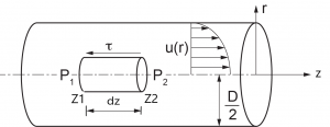
To demonstrate the derivation of the relation for , we consider a laminar flow of a viscous incompressible fluid in a pipe (so-called Hagen-Poiseuille flow) and write Newton’s second law for a cylindrical differential control volume of the fluid with length  along the pipe axis and a cross-section with radius
  , as shown in Figure 8‑3. This flow is axisymmetric, and the velocity profile changes along the radius related to a cylindrical coordinate system
For a steady flow (i.e., non-transient), we have 
 . But the forces applied on the fluid are due to pressures
  at point
  and
and  at point
  and the viscous-induced shear stress
  . Hence,
  where is the radial dimension in the
  plane parallel to the pipe cross-section. We need the relation for fluid friction effect due to viscosity. According to Newton’s law for a viscous fluid, we have
  , assuming the shear stress due to the fluid’s viscosity be proportional to the velocity gradient along the radius with the proportionality constant being the dynamic viscosity
  . Note that velocity profile at any cross-section of the pipe is only a function of radius, or velocity vector is
  . After substitution, we have
  . After simplifying and rearranging the terms, we have
  . Integrating the latter relation, noting that velocity is not a function of
  , gives
  , or
, or  . Now, we rearrange the terms and let
  , the length of the control volume, and use the pressure difference as a positive constant quantity
  in the direction of the fluid flow. Hence,
  . Integrating both sides (the left-hand side with respect to
  and the right-hand side with respect to ) gives
  . The constant of integration can be obtained using the information at the boundary of the pipe assuming the no-slip condition, or
  , where D is the pipe diameter. Therefore,
  . Hence, after back substitution, we get the velocity profile
  . This relation is the famous parabolic velocity profile for the flow in a pipe and can be written in its functional form as
(8.9) 
Using Equation (8.9), we can calculate the velocity for any given value of , e.g.,  at the centre-line of the pipe or at the interior wall of the pipe.
Now, to find the volume flow rate, we integrate the velocity  over the whole cross-section of the pipe using a differential area element
  . Or, the volume of the fluid passing through the whole cross-section of the pipe per unit of time is given by
 , or
, or
(8.10) 
Comparing Equation (8.10) with Equation (8.8), we can write the fluid resistance as
(8.11) 
The fluid resistance can be interpreted as the amount of pressure drop per unit of volume flow rate of the fluid in the pipe. The dimension of fluid resistance can be worked out as ![\Big[\dfrac{kg}{s.m^4}\Big] = \Big[\dfrac{N.s}{m^5}\Big]\equiv \dfrac{pressure}{volume\: flow\: rate}](https://pressbooks.bccampus.ca/engineeringsystems/wp-content/ql-cache/quicklatex.com-2fb967c37fd0bbdb012a7b092c07051a_l3.png "Rendered by QuickLaTeX.com") .
.
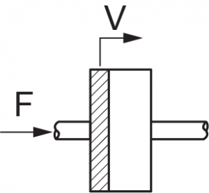
Other BG elements for hydraulic systems are sources of flow (e.g., centrifugal pumps) and efforts (e.g., reservoirs, tanks, displacement pumps). Pumps provide flow of a fluid at a certain flow rate according to their types and specifications. Reservoirs or pressure chambers provide certain pressure to the system as an effort source. The transformers elements are those like piston-cylinder (plunger), and gyrators are those elements like reaction turbines or hydraulic motors. Sketches below show some related elements.
Typical hydraulic components are shown in Table 8‑1.
| -element (valve) |
-element (storage) |
-element (fluid mass) |
 -element -element(plunger) |
 -element -element(pump) |
 |
 |
 |
 |
 |
8.6 Sign Convention for BG Modelling of Hydraulic Systems
The sign convention for hydraulic systems can be defined by specifying the relative high/low pressure points in the system and, hence, the positive fluid flow direction along the pressure drop. The pressure reference is commonly taken to be the atmospheric pressure (i.e., one atm for absolute and zero for gauge pressures). For BG modelling, it is recommended to have all pressures in gauge and define a zero-pressure point for reference atmospheric pressure. If the results are required in absolute pressure units, then one unit of atmospheric pressure can be added to the obtained values from the BG model.
8.7 Guidelines for Drawing BG for Hydraulic Systems
As mentioned in chapter 4, the general guidelines for drawing BG models can be applied to hydraulic systems, along with causality assignment rules. For hydraulic systems, we follow the guidelines given for electrical systems (see section 7.3) as described in the following steps:
1) Assign sign convention for fluid flow directions.
2) Assign 0-junction for each distinct pressure point in the system.
3) Assign 1-junction for each element in the system. This is for taking care of relative pressure drops related to each element located between two adjacent 0-junctions, since 1-junction is effort summator.
4) Select a node in the system as a reference, i.e., the atmospheric pressure point, and assign a 0-junction element to it. If gauge pressures are used, then this 0-junction and all connected power bonds can be eliminated to simplify the model.
5) Assign -element for storage/capacitors, -element for friction, -element for fluid mass, and  for pressure and
  for flow sources.
6) Assign -element for hydraulic transformers and -element for hydraulic gyrators.
7) Connect the elements with power bonds and assign causalities. Simplify by neglecting the bonds and the 0-junction which are connected to the 0-junction representing the atmospheric pressure.
Similarly, a 1-junction-based approach can be used for distinct flow rates and hence simplifying the BG model, as we demonstrated in the previous chapter with electrical systems.
8.8 Example: Hydraulic Reservoir-Valve System
Figure 8‑4 shows a hydraulic system consisting of two tanks, pipes, and valves. Build a BG model for this system.
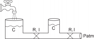
Solution:
We follow the systematic procedure for building the BG model, listed in section 8.7. For this system, we can easily identify two pressure points located at the bottom of tanks. We assign two 0-junctions for each. For flow input, we assign a flow source element, and for the output, an effort source element to define the atmospheric pressure at that location. For the tanks, we only consider capacitance, assuming slow fluid motion and neglect inertia and friction (i.e., no inertance nor resistance). For the pipe sections, we consider inertance and resistance. As well, we assign 1-junctions for flows in the pipes that represent the pressure changes for these components. Figure 8-5 shows the resulting BG model.

8.9 Example: Hydraulic Reservoir-Valve System Simulation
In this example, we use the BG model developed in section 8.8, along with data assigned to parameters for simulation. Considering water as the fluid ( ) and the data given in Table 8‑2, we can calculate the related , , and of the elements in the system. The diameter of the pipes is 15 cm, and
  .
.
The following video shows how to build and run the model for this example in 20-sim.
| Component |  -section area -section area[  ] ] |
Length [  ] ] |
[  ] ]Eq. (8.1) |
[  ] ]Eq. (8.5) |
[  ] ]Eq. (8.11) |
| Storage tanks | 2 | – |  |
– | – |
| Pipe1 | 0.01767 | 4 | – | 226372.4 | 322 |
| Pipe2 | 0.01767 | 2 | – | 113186.2 | 161 |
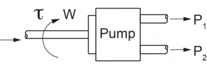
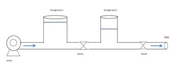
8.10 Example: Hydraulic Pump-Reservoir-Valve System
In this example, we use the BG model developed in section 8.8, adding a pump to the system as shown in Figure 8‑6. In this example we discuss in more detail the BG model of a pump. For further details related to BG modelling of pumps, consult with references cited as [21] and [29].
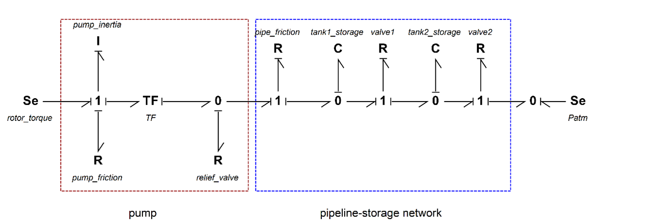
The following video shows how to build and run the model for this example in 20-sim. The resulting BG model is shown in Figure 8‑7.
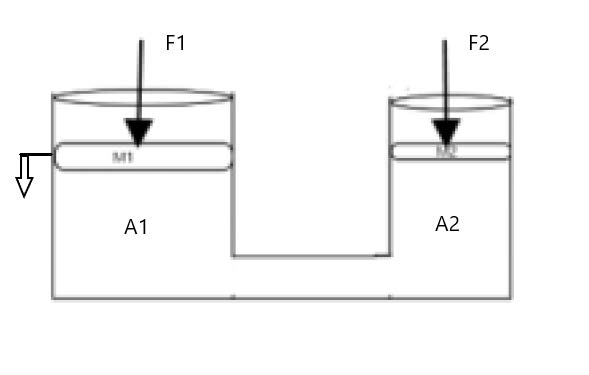
8.11 Example: A Hydraulic Lift System

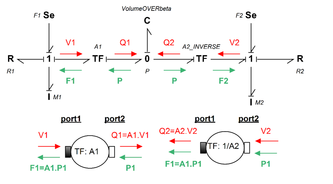
In this example, we consider a hydraulic lift, as sketched in Figure 8‑8. We build a BG model for this hydraulic system. The continuity relation applies to the fluid motion and Pascal’s law defines the pressure distribution of the fluid in the cylinders. Two transformer elements are used in the BG model to convert linear velocities of the pistons to/from volume flow rate and convert forces to pressures (see Figure 8‑9). The transformers’ parameters are explained in the video clip.
The following video shows how to build and run the model for this example in 20-sim.
The BG model is shown in Figure 8‑9, along with the detail of the transformers’ inputs and outputs.
Exercise Problems for Chapter 8
Exercises
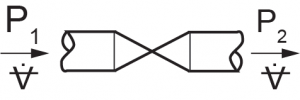
- Build the bond graph for a two-way safety valve.
- Repeat the example in section 8-9 and perform a parametric sweep for some parameters in the simulation, for example pipe diameters and lengths.
- Expand the BG model given in section 8.10 with running simulation with some data for the system parameters, similar to those given in section 8.9. Also, expand the model of the pump using some pump-chart (H-Q).
- Use some data and run simulation for the example given in section 8.11, the hydraulic lift.
Media Attributions
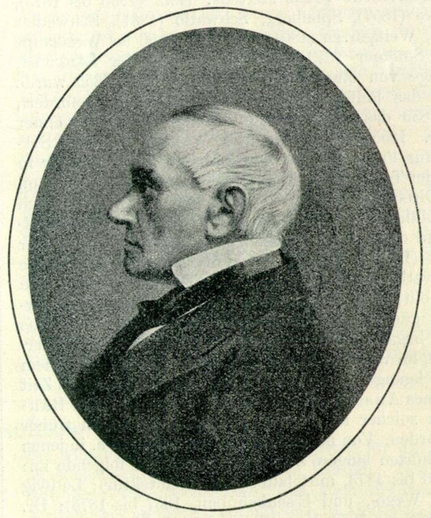
- Gotthilf Hagen © Centralblatt der Bauverwaltung, 1899, S. 237 is licensed under a Public Domain license
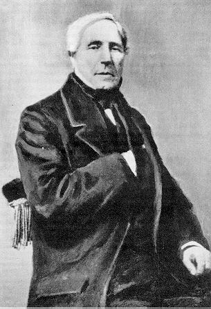
- Jean-Léonard-Marie Poiseuille is licensed under a Public Domain license
- fig-8-3_edits
- Fig-8-4
- Blaise Pascal © Janmad is licensed under a CC BY (Attribution) license
