Bond Graph Modelling Method

Mehrzad Tabatabaian

3 Bond Graph Modelling Method

3.1 Overview

All engineering systems share the physical phenomenon of the transfer and distribution of energy among their corresponding components while converting one form of energy to another. The balance of energy “flowing” through a system should be maintained. The total amount of energy remains constant—energy is conserved—according to the first law of thermodynamics. In 1959, Henry Paynter used the first law and common system features to create a general graphical method for analyzing and modelling multi-domain engineering systems. His objectives were mainly to have a unified graphical method for modelling single- and multi-domain systems as well as a common procedural algorithm to develop such models and obtain their relevant systems’ equations. Hence, the bond graph (BG) method was created [1], [20], [21], [22].

BG represents a system through graphical modelling. The BG method assigns ports (the communication point) for each component of a system and connects each port to the adjacent component through bonds (the communication path and direction) for a two-way energy/power exchange. At any instant of time, each component either receives (sends) a quantity called effort and simultaneously sends (receives) another quantity called flow. The product of the quantities of effort and flow has the dimension of power—or time rate of energy change. In a mechanical system, force is the effort and velocity is the flow; in an electrical system, voltage is the effort and current is the flow. The collection of bonds—with the inclusion of the related system components’ constitutive laws, constraints, and boundary conditions—forms the system BG model. Building a BG model requires nine basic elements, defined as follows. See section 3.4 for full description.

The nine basic BG elements, along with the principle of causality, can be employed for building a BG model representing a given system’s dynamical behaviour (see further sections for detailed explanation). The resulting BG model, then, would clearly show the kinematic (i.e., continuous stream of flow) and kinetic (i.e., continuous stream of effort) of the system and can be used to extract the equations governing the dynamical behaviour of the whole system. In addition, the insights provided by a BG model are valuable for understanding the physics/dynamics of the system and provide a powerful tool for simulation, design, and optimization of the system. The procedure for building a BG model is similar for analogous engineering systems. For example, when the parameters of the pertinent components are used, the BG model for a mechanical mass-spring-damper system is identical to those of an electrical resistor-capacitor-inductor (RCL) system.

In this chapter, we discuss, among other topics, the definitions for basic BG elements, the causality principle and assignments, and the concept of state variables.

3.2 Categorizing System Components—Generalized Effort and Flow

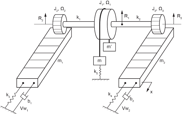
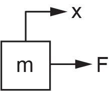
The components of a system can be categorized according to energy transfer through the system into three types. These are kinetic energy storages, potential energy storages, and energy dissipaters. In addition, we have energy source/sink components acting with the surroundings at the boundary of the system. There may also exist components that simply transfer energy without storing or dissipating it. Finally, a system may include components, such as a distributor, that perform as junctions. Figure 3‑1 shows a sketch of a mechanical system with examples of component categories, as mentioned above. All these types of components can be modelled using nine basic BG elements, as discussed in further sections.

Figure 3-1 Sketch of a mechanical system with components’ category types

The dynamical behaviour of a system changes with time. Therefore, time rate of energy or power is the quantity of interest in BG models. The relation between energy $\mathcal{E}$ and power $\mathcal{P}$ can mathematically be written as

(3.1) $\begin{equation*} \mathcal{P} (t) = \frac{d \mathcal{E} (t)}{dt} \quad or \quad \mathcal{E} (t) = \int \mathcal{P} (t)dt \end{equation*}$

We can identify the components of a given system as “lumped” entities that exchange energy with one another. Using the first law of thermodynamics, we can write the change in energy as the sum of work $\mathcal{W}$ and heat $\mathcal{Q}$ exchanges, or $d \mathcal{E} = \mathcal{P} dt = \delta \mathcal{W} + \delta \mathcal{Q}$ . Summing up the energy changes of lumped components in a system gives the total energy change of the system. For example, without losing generality, we consider a mechanical system component receiving power and exhibiting a displacement $x(t)$ and velocity $v(t) = \dfrac{dx}{dt} = \dot x(t)$ . Using Equation (3.1), the amount of energy in terms of work input can be written as $\mathcal{W} = \int \mathcal{P} dt$ . But the work is also equal to the force times the displacement; hence, $\mathcal{W} = \int F(t)dx$ . Substituting for $dx = v(t)dt$ , we get $\mathcal{W} = \int Fvdt$ . Considering $t_1$ and $t_2$ as the time limits associated with the duration of energy transfer, we can, after integrating, write the work as

(3.2) $\begin{equation*} \begin{dcases} \Delta \mathcal{W} |_\textit{potential} = \int_{t_1}^{t_2} F \left( \underbrace{vdt}_{dx} \right) = Fx|_{t_2}-Fx|_{t_1} \\ \Delta \mathcal{W} |_\textit{kinetic} = \int_{t_1}^{t_2} v \left( \underbrace{Fdt}_{dp} \right) = \int_{t_1}^{t_2} v(mdv) = \frac{m}{2} (v^2 |_{t_2} - v^2 |_{t_1}) \\ \Delta \mathcal{W} |_\textit{dissipation} = \int_{t_1}^{t_2} (Fv)dt = \mathcal{P}|_{t_2} - \mathcal{P}|_{t_1} \end{dcases} \end{equation*}$

where $m$ is mass. In a BG model, each system component is designated by a suitable basic element and associated port(s). Depending on the type of element used, the number of ports could be one, two, or more. The power direction is designated by a half-arrow ( $\longrightharpoondown$ ) which shows the direction of power to or from the port for each element. Traditionally, half-arrows are used in BG models to keep the full-arrow shape for one-way signal data, as in block diagram graphs.

As mentioned above and by Equation (3.2), for mechanical systems, the power is composed of two quantities: force and velocity. In BG method, we generalize this concept and show the power with the product of $e$ and $f$ , the effort and flow, respectively. Hence, the product of effort and flow has the dimension of power, or $\textit{power} = e \cdot f$ . For example, for a rotational motion, $e$ is the torque and $f$ is the angular velocity (see Table 3‑1). In other words, in a BG model, the kinetics of a system is modelled by transfer of the efforts of its components according to the equilibrium, and the kinematics by transfer of components’ flows according to compatibility requirement. We will discuss this feature of BG method, using some examples, in section 4.6.

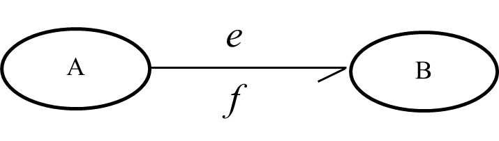
Figure 3‑2 shows the definition of power direction for element A sending power to B, and the associated effort, shown above the half-arrow, and flow, shown, by definition, below the half-arrow.

Figure 3-2 BG power direction and associated effort and flow definitions: B receives power from A

Table 3‑1 Analogous quantity definitions in BG modelling method related to different systems
Systems	Effort ( $e$ )	Flow ( $f$ )	Displacement $q = \int fdt$	Momentum $p= \int edt$
mechanical-translational	force [N]	velocity [m/s]	distance [m]	[kg.m/s]
rotational mechanical	torque [N.m]	angular velocity [rad/s]	angle [rad]	angular momentum [kg.m2/s]
hydraulic	pressure [Pa]	volume flow rate [m³/s]	volume [m³]	hydraulic momentum [Pa.s]
thermal/thermodynamics	temperature [K]	entropy change rate [J/ K.s]	entropy [J/K]	—
thermo-fluid	enthalpy (specific) [J]	mass flow rate [kg/s]	mass flow [kg]	flow momentum
electrical	voltage [V]	current [A]	charge [C]	flux linkage [V.s]
magnetics	magnetic force [A]	magnetic flux rate [Wb/s]	magnetic flux [Wb]	—
chemical	chemical potential [J/mol]	mole flow rate [mol/s]	mole flow [mol]	—

3.3 Causality Principle and Assignment

To establish the principle of cause and effect relationship in BG method, we use the definition of causality assignment. The cause signal brings all the history data to the system/element, and through the dynamical behaviour of the system, the present signal effect is decided and provided as output.

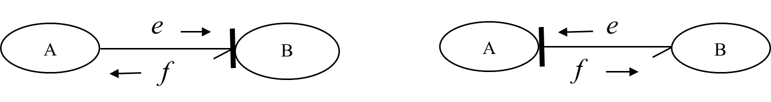
As mentioned, in BG method, the half-arrow indicates the direction of power between related elements in a BG model. However, the half-arrow does not provide information about the direction of power constituents, i.e., effort or of the flow. In principle, we can arbitrarily define these directions. For example, in Figure 3‑2, we can assign $e$ direction pointing from component A to B (hence, $f$ should be directing from B to A) or vice versa. In other words, the causality assignment is a symmetrical one. By definition, a small transverse/vertical line, a causality stroke, is drawn close to one of the ports at the power bond to show the direction of effort toward it, hence the direction of flow away from it, as shown in Figure 3‑3. This operation is critical for building BG models and, in terms of providing a definite solution, has consequences in the resulting equations of the system. After the causality is assigned, then the signal received by the element is the cause, and the returning signal—or the element response—is the effect.

The preferred causality assignment is called integral causality, and the alternative option is the derivative/differentiate causality. We will discuss the details further in section 3.5.

Figure 3-3 Causality assignment definition and directions of effort and flow between elements A and B

3.4 Nine Basic Elements of Bond Graph Method

As mentioned in the previous section, building a BG model of a physical system involves consideration of the energy conservation, transfer, and conversion through the system. In a BG model, we focus on the rate of energy or power as the quantity to deal with.

For energy storage, we define two elements, represented by $I$ (inertial element) for kinetic energy and $C$ (capacity element) for potential energy storages. For energy dissipation, we define one element, represented by $R$ (friction or resistor element). We represent the energy source/sink acting at the boundary of the system by two elements, one for effort $S_e$ and one for flow $S_f$ . To manage the distribution of energy through the system, we define two elements as junctions, represented by junction 1 and junction 0. For energy transfer/conversion, we define two elements, represented by transformer $TF$ and gyrator $GY$ . Therefore, in total, we have nine elements available and sufficient for building a BG for any given physical system, with the inclusion of their modulated versions ( $MS_e$ , $MS_f$ , etc.) for when a signal is input to the corresponding element from an external source. Examples of physical/engineering systems are mechanical, electrical, thermal, hydraulic systems, or some hybrid systems composed of subsystems assembled of different energy media.

Portrait of a Mathematician, thought to be of Robert Hooke (1635–1703)

Each one of the BG elements mentioned above should behave according to the relevant physical laws represented by their constitutive relations—a mathematical model. For example, a linear mechanical spring is modelled by element $C$ , whose governing equation should comply with Hooke’s law. However, a given spring can go under deformation either by receiving an effort (i.e., force) or a flow (i.e., displacement rate/velocity). Depending on the system and computational preferences, we can assign causality strokes to the element $C$ to specify that the desired spring receives effort or flow. This rule, the causality assignment, must be applied to all bonds in a BG model. Examples of typical translational mechanical elements are shown in Table 3‑2.

Table 3‑2 Typical mechanical components and their corresponding BG elements
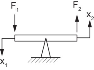
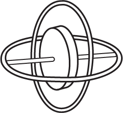
$R$ -element (damper)	$C$ -element (spring)	$I$ -element (mass)	$TF$ -element (lever)	$GY$ -element (gyroscope)

In the next sections, we will define the constitutive equations, preferred causality, and physical representation examples for all nine BG elements.

3.4.1 Inertia Element I: Kinetic Energy Storage

In BG modelling, the $I$ -element is a passive element; it should receive power to return a signal. This requirement means that the half-arrow power bond should be drawn toward this element. An $I$ -element has only one port for communicating to the rest of the system. Examples are mass bodies in mechanical systems and inductors in electrical systems.

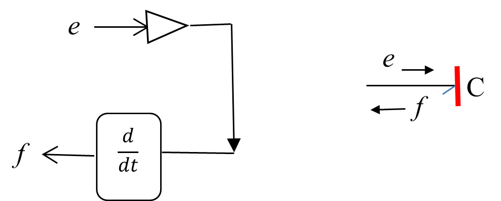
As shown in Figure 3‑4, the input quantity for the $I$ -element can be either effort ( $e$ ) or flow ( $f$ ); consequently, the response is flow or effort, respectively. Note that the causality stroke (the vertical/transverse line) specifies the direction of effort defined to be toward the stroke; hence, the direction of flow is to be away from it. We use red colour for specifying non-integral causality strokes.

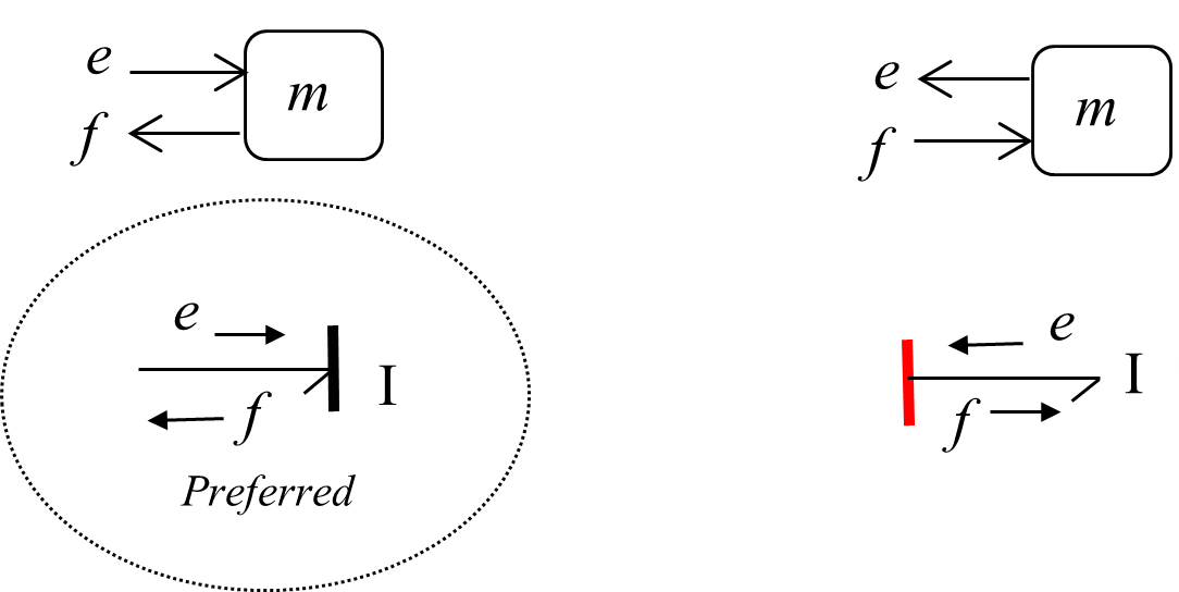Figure 3-4 Causality assignments for an $I$ -element, with preferred integral causality indicated by dashed circle (left) and derivative causality (right)

Now the question is, how do we choose between these two possible options when building a BG model? What are the implications when choosing one option versus the other? The short answer is that both options are legitimate, but there is a preference for having the $I$ -element receiving the effort and sending the flow out—integral causality—hence, the causality stroke is placed at the half-arrow head at the port close to the element. The effort is the cause, and the flow is the effect relevant to $I$ -element when it is integrally causalled.

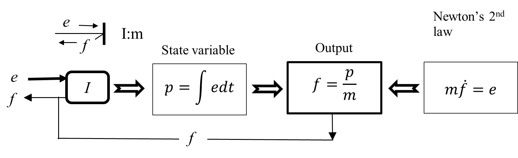
In a bond graph model for an $I$ -element, the preferred causality assignment is effort-in, so-called integral causality.

Mathematically, the statement given in the box can be analyzed as follows. In a mechanical system, for example, we consider a point mass $m$ and apply Newton’s second law to the motion of that point mass. Therefore, we can write ${F}={m}\dfrac{dv}{dt}={m}\dot{v}$ ( $F$ is net applied force, and $v$ is the velocity of the mass), or in BG generalized notation, ${e}={I}\dfrac{df}{dt}={I}\dot{f}$ . Recall that the $e$ symbol represents effort (force) and $f$ represents flow (velocity) in a mechanical system (see Table 3‑1). We also use the symbol $I$ , representing mass $m$ , or inductance for electrical systems. Now, for the effort-in option that we have, since the input should be $e$ , $e ={I}\dot{f}\Rightarrow\underbrace{\dot f}_{output}=\underbrace{\dfrac{e}{I}}_{input}$ or after integration, $\int\dot{f}{dt}=\dfrac{1}{I}\underbrace{\smallint e\:dt}_{momentum}\Rightarrow{f}=\dfrac{p}{I}.$ Note that the integral of force with respect to time is the momentum $p$ , ( $\smallint{F}{dt}=\smallint{edt}$ ). The equation ${f}=\dfrac{p}{I}$ is the key point here. Let’s see what it means. The flow (velocity) is equal to momentum divided by the mass. This is well-known! In BG method, however, it has an important meaning: for the $I$ -element, the input effort quantity, after being integrated, is divided by the $I$ -element parameter $m$ , and the output quantity is flow or velocity. This can be shown in a block/signal diagram along with equivalent BG model diagram (see Figure 3‑5). Since the integration of effort is involved, we call the related causality assignment an integral causality which is preferred for $I$ -elements. From the physical point of view, the integration of effort collects all the input data and hence represents a more comprehensive description of the system in terms of modelling. In addition, the resulting system’s equations (see section 3.5) are first-order ODEs when integral causality is assigned.

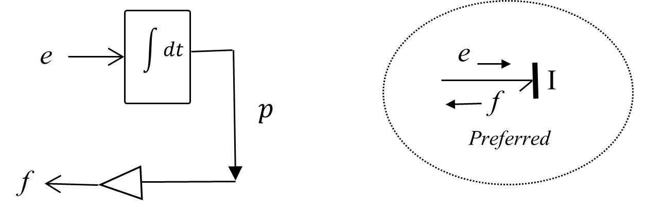Figure 3-5 Block diagram (left) and equivalent bond graph for $I$ -element with assigned integral causality and state variable $p$

The constitutive equation for the $I$ -element in a BG model is given as

(3.3) $\begin{equation*} f={\frac{p}{I}}={\frac{1}{I}}\underbrace{\int e\:dt}_{state\:var.} \end{equation*}$

The momentum $p$ , which is the result of input/effort integration, is a state variable (see section 3.5).

Now, we consider the second possible option with flow-in signal (see Figure 3‑4). We have $e=I\dot{f}=I\dfrac{df}{dt}$ . This equation matches with the input and output data, since the time derivative of input flow, given on the right-hand side of the relation, multiplied by the $I$ -element parameter is the element output or effort, given on the left-hand side. This is the derivative causality assignment since the derivative of input data is involved. This case can be shown in a block diagram along with equivalent BG model diagram (see Figure 3‑6).

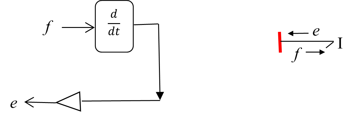Figure 3-6 Block diagram (left) and equivalent bond graph for an $I$ -element with assigned derivative causality

3.4.2 Capacity Element C: Potential Energy Storage Element

In BG modelling method, the $C$ -element is a passive element because it should receive power to react to. This requirement means that the half-arrow power bond should be drawn toward this element. A $C$ -element has only one port for communicating to the rest of the system. Examples are springs in mechanical and capacitors in electrical systems. As shown in Figure 3‑7, the input quantity can be either effort ( $e$ ) or flow ( $f$ ); consequently, the response is flow or effort, respectively. Note that the causality stroke (the vertical line) specifies the direction of effort defined to be toward the stroke; hence, the direction of flow is to be away from it.

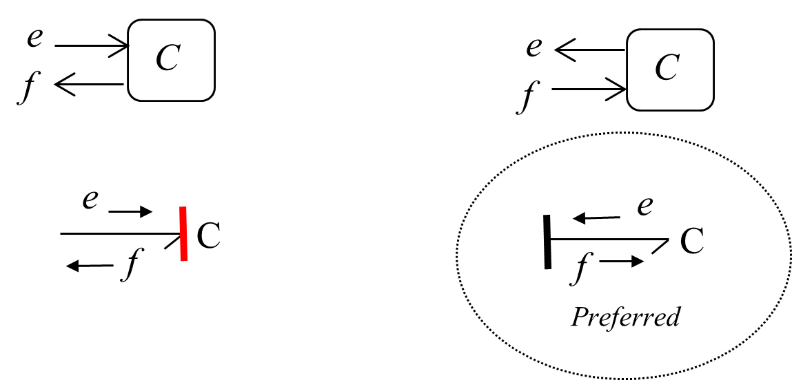Figure 3-7 Causality assignments for a $C$ -element, with preferred one indicated by dashed circle, integral causality (right) and derivative causality (left)

Now the question is, how do we choose between these two possible options when building a model? What are the implications when choosing one option versus the other? The short answer is that both options are legitimate, but there is a preference for having the $C$ -element sending the effort and receiving the flow—integral causality—hence, the causality stroke is placed at the opposite end of the half-arrow head away from the element’s port.

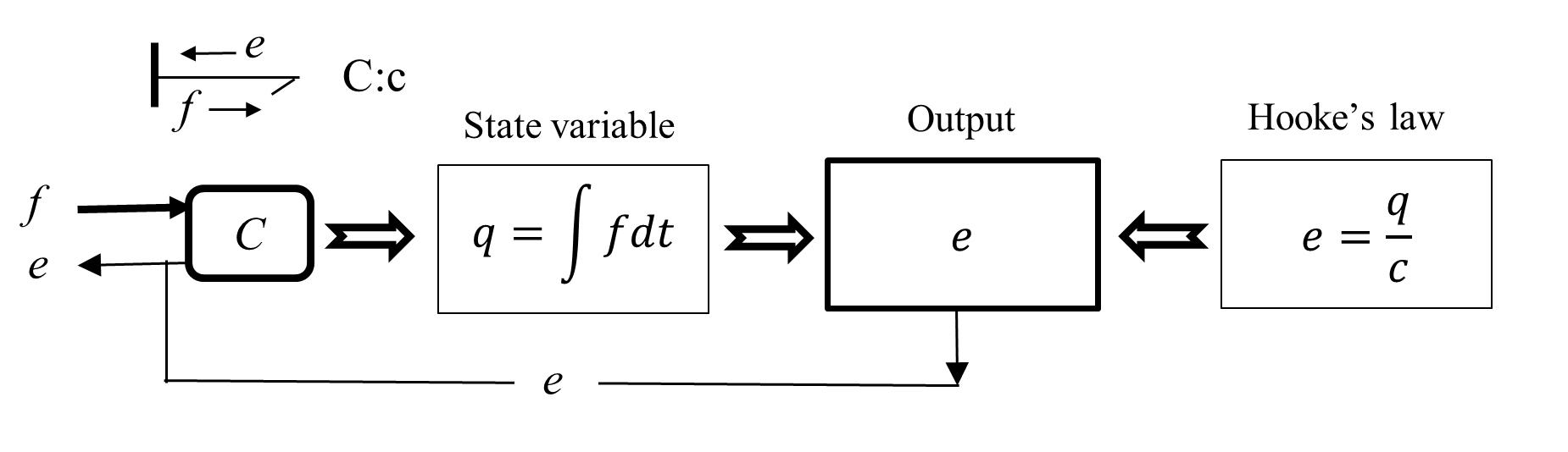
In a bond graph model for a $C$ -element the preferred causality assignment is effort-out, so-called integral causality.

Mathematically, the statement given in the box can be analyzed as follows. In a mechanical system, e.g., we consider a linear mechanical spring with stiffness^[1] $k$ and apply Hooke’s law to its motion. Therefore, we can write $F=kx$ ( $F$ is net applied force, and $x$ is the displacement) or, in generalized BG notation, $e=kq=\dfrac{q}{c}$ , where $c=1/k$ the spring compliance^[2]. Recall that the $e$ symbol represents effort (force) and $f$ represents flow (velocity) in, e.g., a mechanical system, (see Table 3‑1). We use the symbol $c$ , representing spring compliance or capacitance in electrical systems as well.

Now, for the effort-out option having the flow $f$ as the input, we can write $e=\dfrac{q}{c}=\dfrac{1}{c}{\int f\:dt}$ . That is, for the $C$ -element, the input flow quantity, after integration, is divided by the $C$ -element’s compliance and gives the output quantity as effort $e$ . For $C$ -element, the displacement $q$ , which is the result of input/flow integration, is the state variable.

(3.4) $\begin{equation*} e=\frac{q}{c}=\frac{1}{c}\underbrace{\int{f}\:dt}_{state\:var.} \end{equation*}$

This can be shown in a block/signal diagram along with equivalent BG model diagram (see Figure 3‑8).

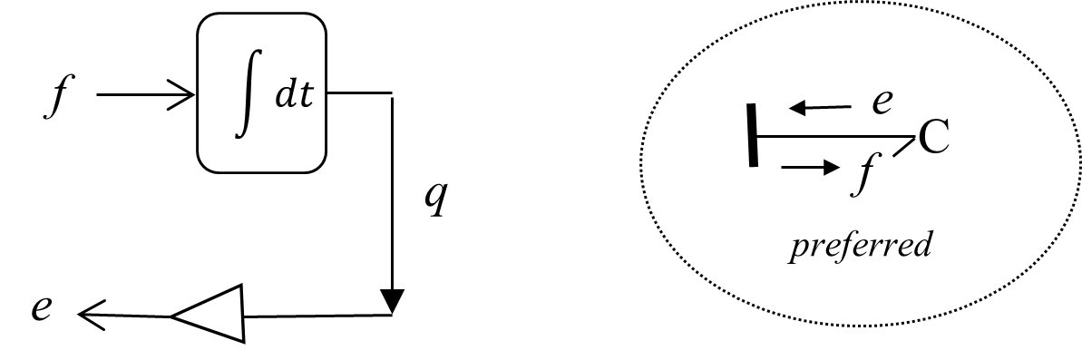Figure 3-8 Block diagram (left) and equivalent bond graph for a $C$ -element with assigned integral causality and state variable $q$

Now, we consider the second possible option with effort-in signal (see Figure 3‑7). We can write $q=ce$ , with effort being the input and displacement as the output data; hence, the time derivative of output displacement ( $q$ ) is required to get the flow/velocity. This is derivative causality assignment, since the derivative/differential operation is needed to get the output signal involved. This case can be shown in a block diagram along with equivalent BG model diagram (see Figure 3‑9).

Figure 3-9 Block diagram (left) and equivalent bond graph for a $C$ -element with assigned derivative causality

3.4.3 Friction Element R: Energy Dissipation Element

In BG modelling method, the $R$ -element is a passive element since it should receive power to return a signal. This requirement means that the half-arrow power bond should be drawn toward this element. An $R$ -element has only one port for communicating to the rest of the system. Examples are dampers in mechanical and resistors in electrical systems.

As Figure 3‑10 shows, the input quantity for the $R$ -element can be either effort ( $e$ ) or flow ( $f$ ); consequently, the response is flow or effort, respectively. Note that the causality stroke (the vertical line) specifies the direction of effort defined to be toward the stroke; hence, the direction of flow is to be away from it.

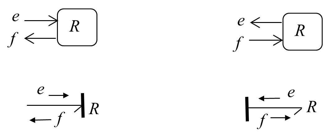Figure 3-10 Causality assignments for an $R$ -element

There is no preference for having the $R$ -element receiving the effort or the flow. Therefore, the causality stroke can be placed at either end of the half-arrow power connection, according to the causality requirement for the adjacent elements.

In a bond graph model for an $R$ -element, there is no preferred causality assignment- i.e., it is neutrally causalled.

Mathematically, the statement given in the box can be analyzed as follows. In a mechanical system, for example, we consider a damper with viscous damping coefficient $R$ . The constitutive equation gives the force applied on the damper proportional to the rate of displacement. Hence, we can write ${F}=Rv$ ( $F$ is net applied force, and $v$ is the velocity). Writing in BG generalized notation, $e=Rf$ . Now, for the effort-in option we have, since the input should be $e$ , $\underbrace{f}_{output}=\underbrace{\dfrac{e}{R}}_{input}$

Now, we consider the option with flow-in data (see Figure 3‑10). We have $e=Rf$ . Since the constitutive equation for a linear viscous damper is algebraic, we do not need to integrate or differentiate the input signal to obtain the output signal for an $R$ -element. Therefore, there is no preference, and $R$ -element is neutrally causalled. Figure 3‑11 shows block diagrams along with equivalent BG model diagram with causality assignments for an $R$ -element.

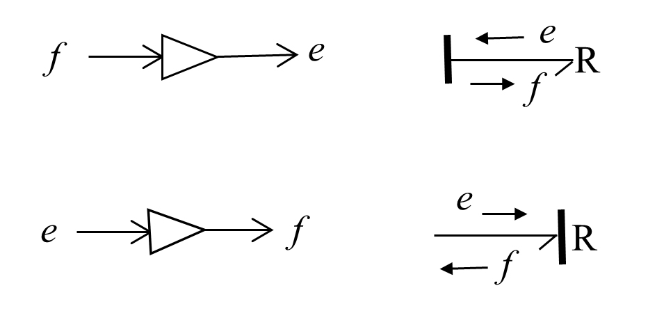Figure 3-11 Block diagrams (left) and equivalent bond graph for an $R$ -element with assigned causality

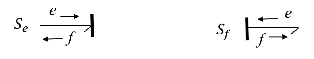
3.4.4 Source Elements S_e and S_f : System Boundary Input Elements

In BG modelling method, the boundary source elements are of two types. The sources for effort (such as force, voltage) and flow (such as velocity, current) are represented by $S_e$ and $S_f$ respectively. These elements are active, and the half-arrow power bond should be drawn from these sources to the connecting elements in the system. Source elements have only one port each, for communicating to the rest of the system. As shown in Figure 3‑12, the causality assignments are uniquely assigned for these elements.

Figure 3‑12 BG symbols for effort source (left) and flow source (right) with their assigned causalities

3.4.5 1- and 0-junctions: Distribution Constraint Elements

In BG modelling method, system-required constraints for distribution of energy are applied using two elements. These are multi-port elements with symbols “1” and “0” that can receive or send power to the elements connecting to them. This requirement means that the half-arrow power bond can be drawn toward or from these elements.

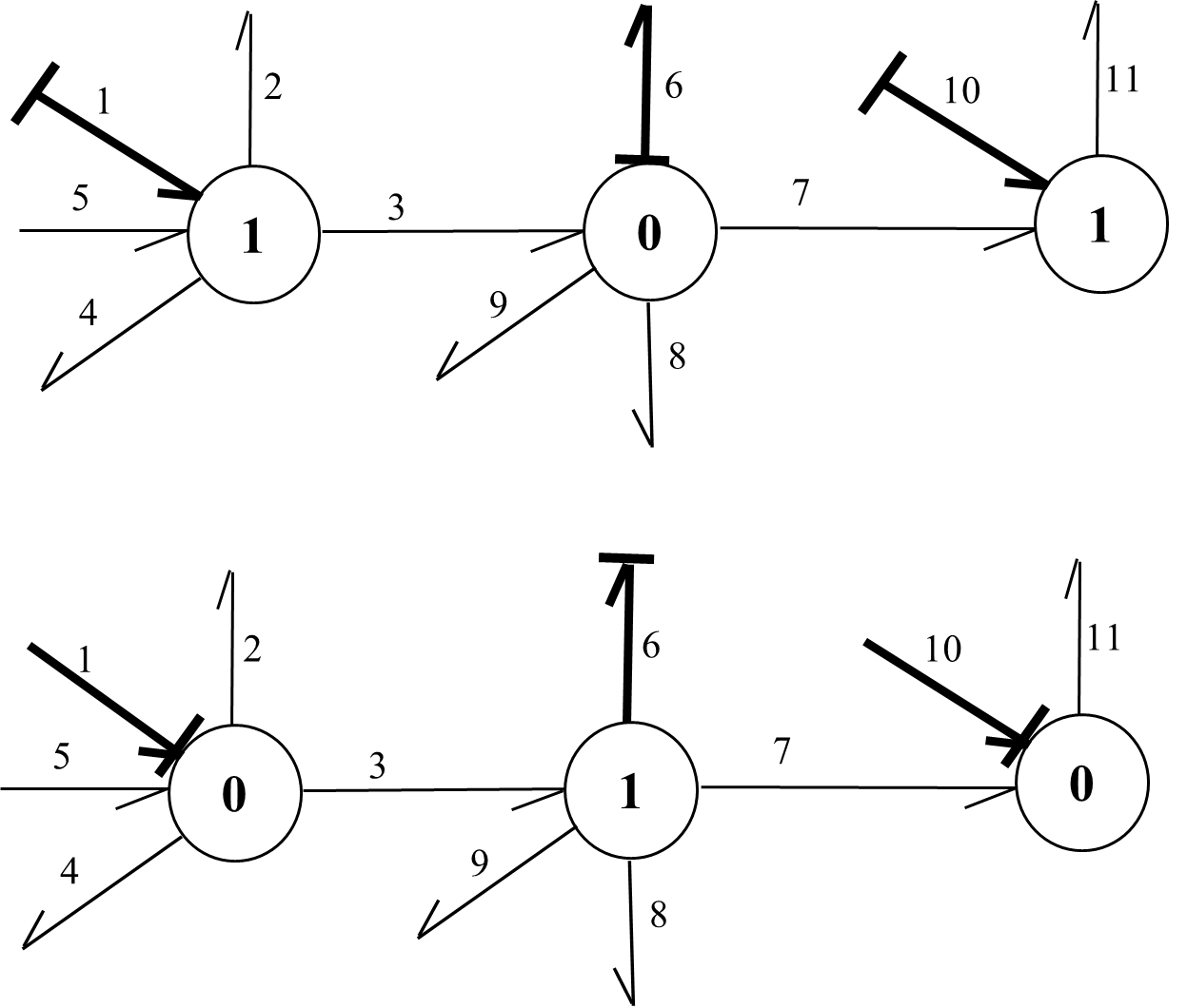
A 1-junction is a flow equalizer or an effort summator element. For example, in a mechanical system, a common node with connecting system components exhibits the same value of velocity, or the elements of an electrical circuit experience the same value of current. The causality assignment for a 1-junction element must comply with its definition of distributing the flow received through one of the connecting bonds to the rest of bonds. Therefore, only one bond can send flow to a 1-junction—the strong bond—and the remaining connecting bonds should send the same flow to connecting elements; hence, the causalities are assigned accordingly, as shown in Figure 3‑13.

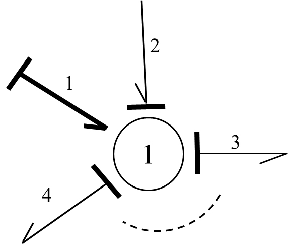
Figure 3‑13 BG symbol for 1-junction element with four connecting bonds, corresponding causalities, and strong bond identified with thick half-arrow

After labelling the bonds with arbitrary numbers, we can write the conservation energy law, in terms of its rate, as $e_1 f_1 + e_2 f_2 - e_3 f_3 - e_4 f_4 = 0$ . But the 1-junction distributes the flow received from the strong bond (i.e., the bond labelled “1”) equally to bonds 2, 3, and 4. Hence, $f_1 = f_2 = f_3 = f_4$ . From these relations, after substitution, we get $e_1 + e_2 - e_3 - e_4 = 0$ . Similarly, for $N$ number of bonds connecting to a 1-junction, we have the constraint relations for the 1-junction as

(3.5) $\begin{equation*} \begin{dcases} f_1 = f_2 = \cdots = f_N \\ \sum_{i=1}^{N} e_i= 0 \end{dcases} \end{equation*}$

In Equation (3.5), the summation for efforts received by 1-junction is algebraic, or the input power is considered to be positive, and the output power has a negative sign.

A 0-junction is an effort equalizer or a flow summator element. For example, in a mechanical system, a common node with connecting system components experiences relative velocity values or the nodes in an electrical circuit with common voltage. The causality assignment for a 0-junction element must comply with its definition of distributing the effort received through one of the connecting bonds to the rest of bonds. Therefore, only one bond can send effort to a 0-junction—the strong bond—and the remaining connecting bonds should send the same effort to connecting elements, hence, the causalities are assigned accordingly, as shown in Figure 3‑14.

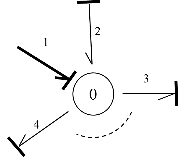
Figure 3‑14 BG symbol for a 0-junction element with four connecting bonds, corresponding causalities, and strong bond identified with thick half-arrow

After labelling the bonds with arbitrary numbers, we can write the conservation energy law, in terms of power or energy rate, as $e_1f_1+e_2f_2-e_3f_3-e_4f_4=0$ . But the 0-junction distributes the effort received from the strong bond (i.e., the bond labelled “1”) equally to bonds 2, 3, and 4. Hence, $e_1=e_2=e_3=e_4$ . From these relations, after substitution, we get $f_1+f_2-f_3-f_4=0$ . Similarly, for $N$ number of bonds connecting to a 0-junction, we have the constraint relations for the 0-junction as

(3.6) $\begin{equation*} \begin{dcases} e_1=e_2=\cdots=e_N\\ \sum_{i=1}^{N} f_i=0 \end{dcases} \end{equation*}$

In Equation (3.6), the summation for flows received by the 0-junction is algebraic, or the input power is considered to be positive and the output power has a negative sign.

3.4.6 Transformer TF and Gyrator GY: Energy Conversion Elements

In physical engineering systems, energy may be converted by some components while its conservation is maintained. Examples are levers and gearbox in mechanical systems or electrical transformers and motors in electrical systems. In BG modelling method, there exist two elements for modelling convertors: transformer $TF$ and gyrator $GY$ . These elements are two-port elements and can receive power through one of their ports as input and deliver a converted power from the other port as output, in terms of the power variables effort and flow. The causality assignments determine the directions of flows and efforts as being inputs or outputs. In this section, we present the details of $TF$ -element followed by those of $GY$ -element.

A transformer element, $TF$ represents the converter that receives the same type of physical quantity as the type it delivers, after conversion. For example, a force applied at one end of a lever is converted to a magnified/reduced force at the other end, or the velocity of the lever’s end point is converted to another velocity value related to another point proportional to their distances from the lever’s pivot.

As shown in Figure 3‑15, a $TF$ -element can have one effort and one flow as inputs, and consequently, delivers converted corresponding effort and flow as outputs. The conversion parameter $\lambda$ should be defined, based on the physical system data. For example, for the case that flow $f_1$ is the input and flow $f_2$ the output, we can write $f_2 = \lambda f_1$ to define $\lambda$ . But from energy conservation we have $e_1 f_1 = e_2 f_2$ , or the output effort $e_1 = \underbrace{(f_2/f_1)}_{\lambda}e_2 = \lambda e_2$ . Similarly, for the case that effort $e_1$ is the input and effort $e_2$ the output, we can write $e_2 = \lambda^{-1} e_1$ , using $\lambda$ . But from energy conservation, we have, $e_1 f_1 = e_2 f_2$ or the output flow $f_1 = \underbrace{(e_2/e_1)}_{{1}/\lambda}f_2 = \lambda^{-1} f_2$ .

These relations constitute the $TF$ -element equations and are shown in Figure 3‑15, for each case where the inputs to the $TF$ -element are identified with thick arrows.

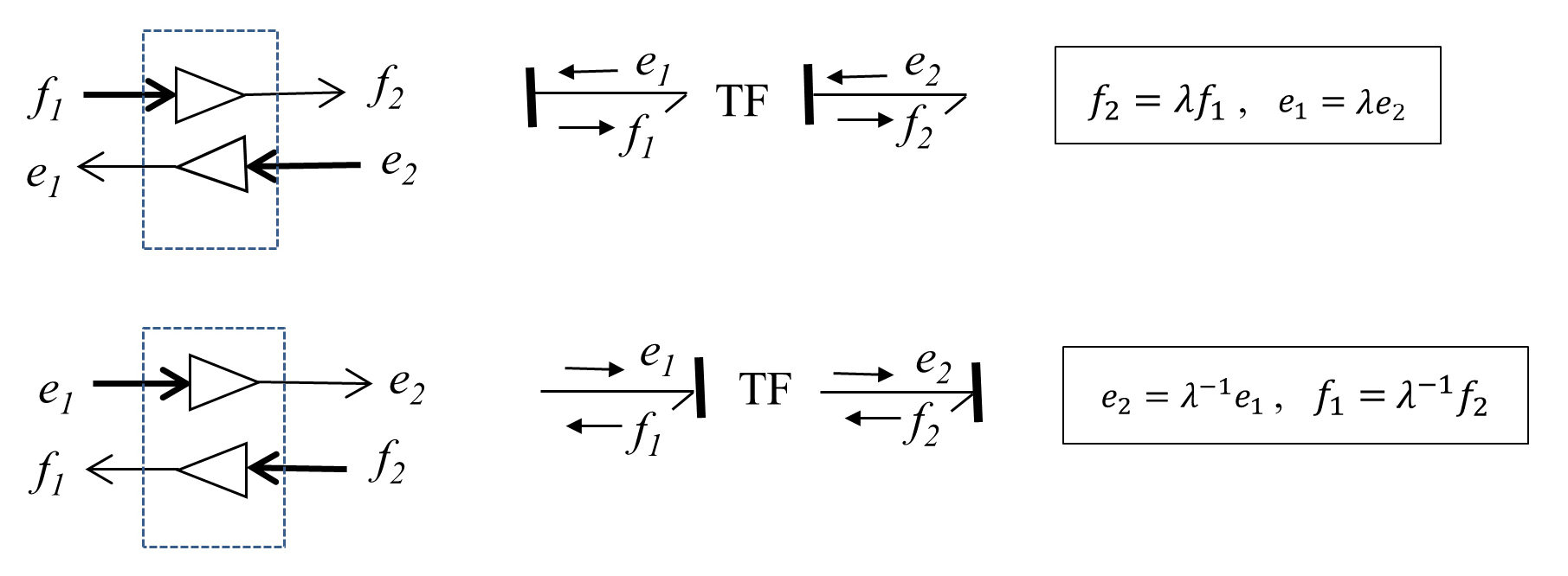Figure 3-15 Block diagrams (left) and equivalent bond graphs for a $TF$ -element with related assigned causalities—inputs are shown with thick arrows

Note that the $TF$ -element should have only one of the two required causality strokes near it for either cases, as shown in Figure 3‑15.

In a bond graph model for the $TF$ -element, there should be only one causality stroke close to it and another one away from it. A $TF$ -element converts flows to flows and efforts to efforts.

A gyrator element, $GY$ , represents the converter that receives a type of physical quantity and delivers a different type after conversion. Examples are a DC motor which converts voltage (effort) to angular velocity (flow) of the rotor or the attached shaft. The reverse operation is that of an electric generator.

As Figure 3‑16 shows, a $GY$ -element can have one effort and one flow as inputs and, consequently, delivers corresponding flow and effort as outputs. The conversion parameter $\kappa$ should be defined, based on the physical system data. For example, for the case with flow $f_1$ as the input and effort $e_2$ being the output, we can write $e_2 =\kappa f_1$ to define $\kappa$ . But from energy conservation we have $e_1 f_1 = e_2 f_2$ , or the output effort $e_1 = \underbrace{(e_2/f_1)}_{\kappa}f_2 = \kappa f_2$ . Similarly, for the case with effort $e_1$ as the input and effort $f_2$ being the output, we can write $f_2 = \kappa^{-1} e_1$ , using $\kappa$ . But from energy conservation we have $e_1 f_1 = e_2 f_2$ , or the output effort $e_1 = \underbrace{(e_2/f_1)}_{\kappa} f_2 = \kappa f_2$ . Similarly, for the case with effort $e_1$ as the input and effort $f_2$ being the output, we can write $f_2 = \kappa^{-1}e_1$ , using $\kappa$ . But from energy conservation we have $e_1 f_1 = e_2 f_2$ , or the output flow $f_1 = \underbrace{(f_2/e_1)}_{1/ \kappa} e_2 = \kappa^{-1}e_2$ . These relations constitute the $GY$ -element equations and are shown for each case where the inputs for the $GY$ -element are identified with thick arrows in Figure 3‑16.

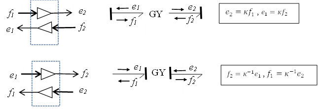
Figure 3-16 Block diagrams (left) and equivalent bond graphs for a $GY$ -element with related assigned causalities—inputs are shown with thick arrows

Note that the $GY$ -element should have both required causality strokes near it or away from it, as shown in Figure 3‑16.

In a bond graph model for the $GY$ -element, there should be two causality strokes close to it or both away from it. A $GY$ -element converts flows to efforts and efforts to flows.

Now that we have all nine elements of BG method defined, in the following sections we discuss the state variables, their definitions, and relation with integral causality. State variables are key quantities in analyzing engineering system dynamics and behaviour and are a critical part of BG method. A sound understanding of the state variables will help in developing a high level of competency in BG method and its applications to engineering systems.

3.5 System State Variables

The main objective of BG models is to derive system equations that describe the behaviour of the system and to follow up by solving these equations for simulation and design purposes.

The system equations may be ODEs of second order or higher. However, when writing these governing system equations in terms of state variables—those variables that uniquely and sufficiently describe the system dynamics—we end up having first-order ODEs, a huge advantage when using numerical/analytical solution methods. In addition, when we extract system equations from the corresponding BG model (see chapter 11), additional algebraic equations are involved; hence, we have a system of differential-algebraic equations (DAEs) that could benefit from having the related ODEs written as first-order equations.

In this section, we define the state variables that relate themselves to the storage elements in BG method i.e., $I$ -element and $C$ -element. Other BG elements correspond to the algebraic equations of the system DAEs and do not possess state variables of their own.

We now consider the kinetic energy storage element or inertia $I$ -element. The energy stored can be written as the integral of power (i.e., effort multiplied by flow) with respect to time, $\int e \cdot f\: dt$ or as $\int e \cdot f\: dt=\int(edt)f$ . But $edt=dp$ , the generalized momentum differential/change. Hence, $\int (edt) f = \int f\: dp$ , or the energy stored in an inertia element $I$ is the integral of flow (e.g., velocity) with respect to momentum as the independent variable. Therefore, a functional form of the type $f = \mathcal{F} (p)$ is required to perform the integral operation. In other words, the area under the curve of the flow $f$ in the $f-p$ coordinate system is equal to the energy stored. Recall that, e.g., in mechanical systems, this function (i.e., $f = \mathcal{F} (p)$ ), is derived from Newton’s second law, or $f = p/I$ (the parameter $I$ is mass or inductance, for example). Therefore, we have $\textit{Energy} =\int f\: dp=\dfrac{1}{I}\int p\: dp=\dfrac{p^2}{2I}$ , or

(3.7) $\begin{equation*} \textit{Energy stored as an I element} = \frac{p^2}{2I} \end{equation*}$

Equation (3.7) clearly shows that the energy stored by an $I$ -element is uniquely defined by its generalized momentum. Therefore, the momentum of an $I$ -element is identified as a state variable of the system.

The generalized momentum associated with Inertia element in the bond graph model is a system state variable, so-called $p$ on $I$ .

Similarly, we consider the potential energy storage element, or $C$ -element. The energy stored can be written as the integral of power with respect to time, $\int e \cdot f\: dt$ or as $\int e \cdot f\: dt=\int(fdt)e$ . But $fdt=dq$ , the generalized displacement differential/change. Hence, $\int(fdt)e=\int e\: dq$ or the energy stored in a $C$ -element is the integral of effort (e.g., force) with respect to displacement as the independent variable. Therefore, a functional form of the type $e= \mathcal{H} (q)$ is required to perform the integral operation. In other words, the area under the curve of $e$ as a function of $q$ in the $e-q$ coordinate system is equal to the energy stored. Recall that, e.g., in mechanical systems, this function (i.e., $e=\mathcal{H} (q)$ ) is derived from Hooke’s law, or $e=q/c$ (the parameter $c$ is spring compliance or capacitor capacitance, for example). Therefore, we have $\textit{Energy} = \int e\:dq=\dfrac{1}{c}\int q\:dq=\dfrac{q^2}{2c}$ , or

(3.8) $\begin{equation*} \textit{Energy stored in a C-element} = \frac{q^2}{2c} \end{equation*}$

Equation (3.8) clearly shows that the energy related to a $C$ -element is uniquely defined by its generalized displacement. Therefore, the displacement of a $C$ -element is identified as a state variable of the system.

The generalized displacement associated with a $C$ -element in the bond graph model is a system state variable, so-called $q$ on $C$ .

These two state variables ( $p$ and $q$ ) are key variables when extracting system equations from the corresponding bond graph (see chapter 11). The total number of independent system equations is equal to the total number of state variables, or $p$ on $I$ and $q$ on $C$ .

The reader should also note that the assumed governing equations for these two elements (i.e., Newton’s second law for $I$ -elements and Hooke’s law for $C$ -elements) determine the functional forms of $f= \mathcal{F}(p)$ for an $I$ -element and $e=\mathcal{H} (q)$ for a $C$ -element, respectively. Other constitutive equations: e.g., non-linear relations could be used if desirable, but the uniqueness of energy stored on the $p$ and $q$ remains for each of these two elements.

3.5.1 Integral Causality and State Variables: I– and C-elements

The main objective of assigning a causality stroke to an element is to make the element definite in terms of its inputs and outputs (i.e., either effort or flow). Since we have two choices (either effort or flow being the input or the output), the preferred causality is the one that, when assigned, allows the input to the element such that the element-related laws of physics are satisfied and the state variable is concluded as well. For example, if an element receives effort, then it should respond with flow, and the related state variable should be the outcome of the application of the laws of physics to this element. These objectives are met when we use the integral causality strokes for $I$ -element and $C$ -element. In other words, when the integral of the cause signal is equal to the state variable of the corresponding storage element, then that element is integrally causalled.

In the previous sections (see sections 3.4.1 and 3.4.2), we discussed the preferred causalities for $I$ – and $C$ – elements as being the integral causality types. Having defined the state variables for $I$ – and $C$ – elements (see section 3.5), we can expand the discussion on why the integral causality is the preferred one for these elements.

The state variable corresponding to elements $I$ and $C$ specifies the assignment of causality strokes for the integral causality is defined such that the integral of input quantity (either effort or flow) for $I$ – or $C$ -elements result in the corresponding state variable.

Recall that generalized momentum $p$ is the state variable for an $I$ -element. Now, we consider the choice of having the flow $f$ or effort $e$ as the input for $I$ -element according to the causality stroke assignment (see Figure 3‑4). When the effort is selected as the input, we can integrate it (hence, the designation of integral causality for this choice), and get the momentum, i.e., the state variable, as well as the flow for the element response. This is consistent with the $I$ -element governing equation (i.e., Newton’s second law). Therefore, having the causality stroke at the port of $I$ -element, or the preferred causality assignment (see Figure 3‑4), satisfies all the mathematical requirements and provides the flow as the response and the momentum as the state variable. The whole process is shown in Figure 3‑17. The choice of having flow as the input for $I$ -element—the derivative causality—does not fulfill all the objectives mentioned above; hence, it is not preferred. Note that when derivative causality is assigned, Newton’s second law still is satisfied, but the state variable is not explicitly involved.

Figure 3-17 Consistency of integral causality assignment and state variable for an $I$ -element with parameter $m$

Similarly, for a $C$ -element, we can have a similar argument. Recall that generalized displacement $q$ is the state variable for a $C$ -element. Now, we consider the choice of having the flow $f$ or effort $e$ as the input for $C$ -element according to the causality stroke assignment (see Figure 3‑7). When the flow is selected as the input, we can integrate it (hence the designation of integral causality for this choice) and get the displacement, i.e., the state variable, as well as the effort as the element’s response. This is consistent with the $C$ -element governing equation, i.e., Hooke’s law. Therefore, having the causality stroke away from the port of $C$ -element, or the preferred causality assignment (see Figure 3‑7) satisfies all the mathematical requirements and provides the effort as the response and the displacement as the state variable. The whole process is shown in Figure 3‑18. The choice of having effort as the input for $C$ -element—the derivative causality—does not fulfill all the objectives mentioned above; hence, it is not preferred. Note that when derivative causality is assigned Hooke’s law still is satisfied but the state variable is not explicitly involved.

Figure 3-18 Consistency of integral causality assignment and state variable for a $C$ -element with parameter $c$

Exercise Problems for Chapter 3

Exercises

Using Figure 3‑1, identify each component in terms of its type related to energy storage, dissipation, converter, and source.
Using Figure 3‑3, explain if the power bond direction and causality stroke assignment are independent from each other or dependent.
List nine basic bond graph elements and sketch them with their preferred causalities, where applicable.
For each bond graph sketch, perform the operations given below:
1. Write the energy rate balance equation at each junction
2. Identify strong power bond.
3. Assign all remaining causality strokes, using red colour to distinguish them
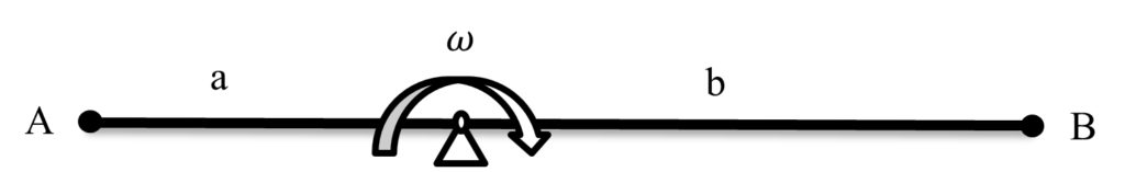
The massless lever rotates about the pivot point with angular velocity , as shown in the below sketch. Draw the bond graph model using TF- element along with equation model for each case:
1. Velocity magnitude at point A is given, $V_A$ . Calculate the transformer parameter $\lambda_V$ .
2. Force magnitude at point A is given, $F_A$ . Calculate the transformer parameter $\lambda_F$
3. Discuss the relation between $\lambda_V$ and $\lambda_F$ .
Describe system state variables and explain their significance related to a system’s equations. Identify BG elements associated with these variables.
Discuss the principle of cause and effect in relation to causality assignment in BG method. For the following elements, assign the causalities and identify the cause and effect for each one. Also identify the integral vs. the derivative causality.